19 Z-test
Why is the \(Z\) distribution so important?
To be candid, for the privileged
Rusers of the world, it really isn’t that essential to our day to day statistical adventures.This is because, if we want to know what \(P(X < x)\) for \(X \sim N(\mu_X, \sigma_x)\) then we just type
pnorm(x, mu_x, sigma_x, lower.tail=TRUE)and let R do all the hard work.But what is R doing under the hood?
Recall that \(P(X < x)\) for \(X \sim N(\mu_X, \sigma_x)\) corresponds to the area under the probability density function in the interval \([-\infty, x]\).
Further recall that the equation that describes the PDF of a normal distribution is given by:
\[ f(x) = \frac{1}{\sigma_X \sqrt(2 \pi)} e^{ -\frac{1}{2} (\frac{x - \mu_X}{\sigma_X})^2 } \]
- This means that \(P(X < x)\) is given by:
\[ P(X < a) = \int_{\infty}^{a} \frac{1}{\sigma_X \sqrt(2 \pi)} e^{ -\frac{1}{2} (\frac{x - \mu_X}{\sigma_X})^2 } \]
It turns out that without awesome computer programs like R, evaluating this integral is challenging.
The old school solution to this challenge was to evaluate this integral for the standard normal (\(Z\)) and put that solution in the back of standard statistics text books in the form of big giant tables.
The \(Z\) distribution has other uses in statistics and machine learning, but most of them are beyond the scope of this unit.
We will see that the overarching idea of the z-transform – i.e., standardising data to mean zero and variance one – comes up when we get to the t-test (later this lecture!).
mu_x <- 90
mu_x_bar <- mu_x
sig_x <- 10

n <- 100
x_obs <- rnorm(n, mu_x, sig_x)

# Using Normal distribution
x_bar_obs <- mean(x_obs)
sig_x_bar <- sig_x / sqrt(n)
px <- pnorm(x_bar_obs, mu_x_bar, sig_x_bar, lower.tail=TRUE)

## Using Z distribution
z_obs <- (x_bar_obs - 90) / sig_x_bar
pz <- pnorm(z_obs, 0, 1, lower.tail=TRUE)

## Compare p-values from different methods
px
## [1] 0.4145534## [1] 0.4145534How are the p-values the same?
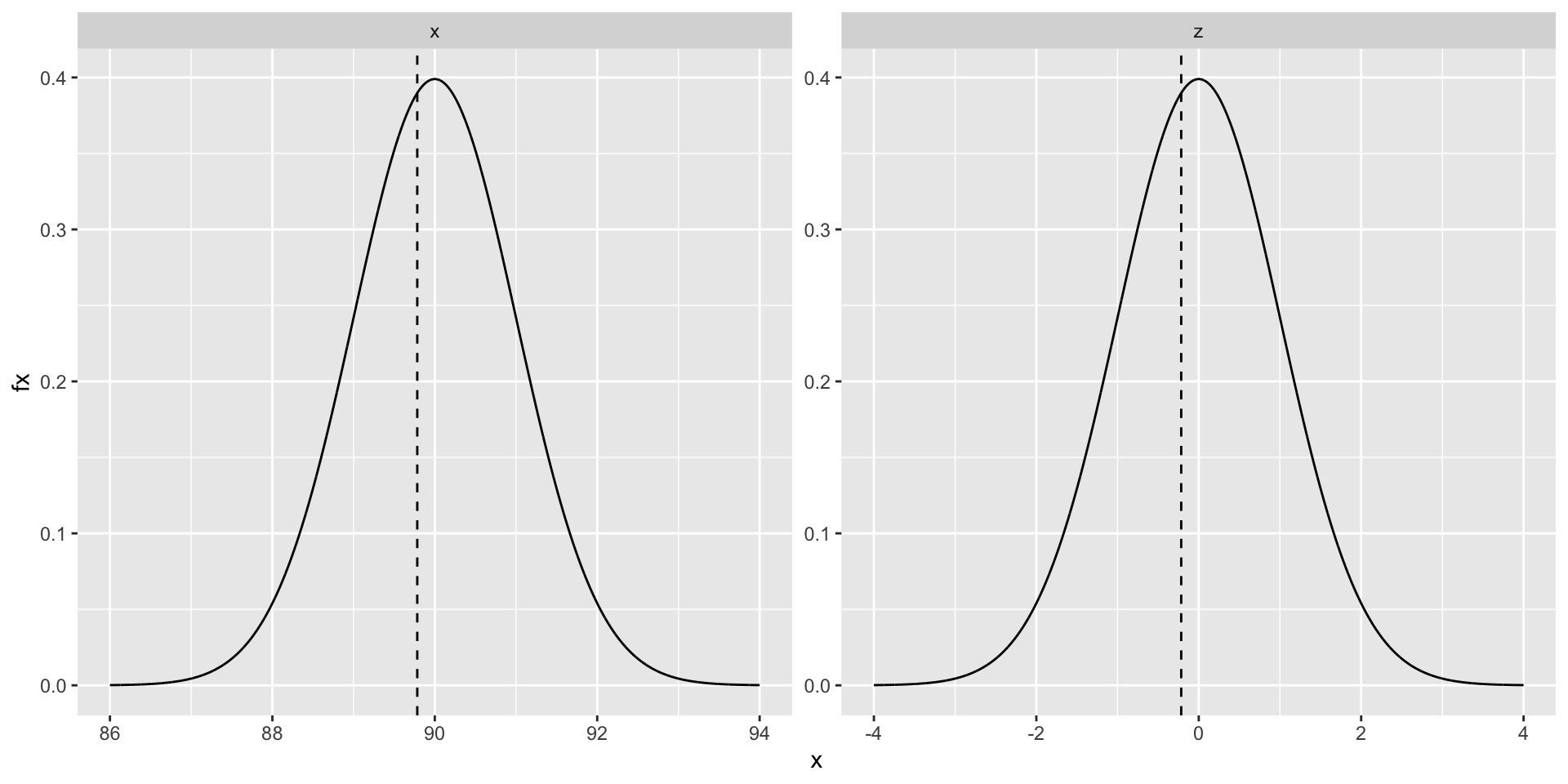
The plot below is the X distribution on the left and the Z distribution on the right. - Notice that the Z is just a scaled version of X, and the that scaling also applied to the observed value.
This means that all probabilities (area under the curve) are the same.
