23 Binomial Test
Consider an experiment in which researchers are trying to determine if a particular rat has learned to press one of two levers whenever they are placed inside of an experimental apparatus. Intuitively, answering this questions would be as simple as just watching the rat and taking note of whether it pressed the correct lever or not. The trouble is that rat behaviour is somewhat random: it sometimes pressed the correct lever and sometimes presses the incorrect lever.
Suppose that the experiment contained \(n=100\) trials and the number of trials in which the rat pressed the lever was \(n_{\text{pressed}}=61\). Did the rat learn or not? We turn to Null Hypothesis Significance Testing (NHST) to answer this question.
1. Specify the null and alternative hypotheses (\(H_0\) and \(H_1\)) in terms of a distribution and population parameter.
First, decide on a statistical model for the measurements you are trying to reason about. That is, think of your data as being samples from a random variable. What distribution does that random variable have? We have a rat that either presses the correct lever or doesn’t. This is a dichotomous outcome, so we know that Binomial distribution is a good model. Recall that the binomial has two parameters, (1) the number of trials \(n\) and (2) the probability of success \(p\). The number of trials is fixed for us by our experiment (\(n=100\)), and \(p\) is the very thing we are trying to reason about. If \(p=0.5\) then the rat is just guessing at the levers. This corresponds to a null result, and therefore to the null hypothesis \(H_0\). If \(p>0.5\) then the rat is doing better than guessing and we would say that it has learned. Therefore, this corresponds to the alternative hypothesis \(H_1\). Let \(X\) be the binomial random variable that generates the results in the above experiment. Then,
\[ X \sim binomial(n=100, p) \\ H_0: p = 0.5 \\ H_1: p > 0.5 \]
2. Specify the type I error rate – denoted by the symbol \(\alpha\) – you are willing to tolerate.
It is traditional in psychology and neuroscience to tolerate a \(5\%\) type I error rate in our inference procedure. This means that 5 out of every 100 times we think the rat has learned, we will have made an incorrect conclusion.
\[ \alpha=0.05 \]
3. Specify the sample statistic that you will use to estimate the population parameter in step 1 and state how it is distributed under the assumption that \(H_0\) is true.
We are trying to make an inference about the population parameter \(p\). An intuitive estimate of this parameter is the proportion of successful trials relative to all trials performed. Let \(x\) be the be the count of successful trials. Then,
\[ \widehat{p}=\frac{x}{n} \]
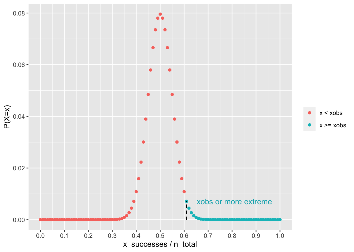
We know that \(X\) is Binomial, but what about \(\widehat{p}\)? With some careful thinking, we can see that \(\widehat{p}\) is also Binomial. The possible outcomes of \(X\) just need to be normalised by the total number of observations \(n\). The probabilities associated with each outcome are the same as those that corresponded to the \(X\) distribution. Another approach (not taken here) is to rephrase the hypotheses to be in terms of counts instead of proportions (e.g., \(H_0: np = 50; H_0: np > 50\)). The sampling distribution of \(\widehat{p}\) under the null is as follows:
\[ \widehat{p} = \frac{X}{n} \sim binomial(n=100, p=0.5), x \rightarrow \frac{x}{n} \]

4. Obtain a random sample and use it to compute the sample statistic from step 3. Call this value \(\widehat{\theta}_{\text{obs}}\)
This was given to us in the formulation of the example. The key is to understand that in this example, \(\widehat{\theta}_{\text{obs}} = \widehat{p}_{\text{obs}}\).
\[ \widehat{p}_{\text{obs}}=\frac{61}{100} \]
5. If \(\widehat{\theta}_{\text{obs}}\) is very unlikely to occur under the assumption that \(H_0\) is true, then reject \(H_0\). Otherwise, do not reject \(H_0\).
Compute the probability of \(\widehat{\theta}_{\text{obs}}\) or a more extreme outcome occurring under the assumption that \(H_0\) is true. This value is called the p-value in NHST. If the p-value is very small (less than ) then reject \(H_0\). Otherwise, fail to reject \(H_0\). Formally, we write our decision rule as follows:
\[ \text{if } P(\widehat{\theta} \geq \widehat{\theta}_{\text{obs}} | H_0) \leq \alpha \rightarrow \text{Reject } H_0\\ \text{otherwise fail to reject } H_0 \]
Notice that our logic only allows to reject or fail to reject the null hypothesis. We can’t make any inference about the alternative hypothesis (e.g., we can’t accept the alternative). We are only assessing the evidence for the null. The purpose of including an alternative hypothesis is to give meaning to what sorts of outcomes correspond to more extreme than what we observed.
To proceed, note again that in this example \(\widehat{\theta}_{\text{obs}} = \widehat{p}_{\text{obs}}\). We therefore need to compute
\[ P(\widehat{p} \geq \widehat{p}_{\text{obs}} | H_0) \]
When actually computing the p-value, we will turn to
pbinom(). From the plot above, and from reasoning about
the alternative hypothesis, we see that we need
lower.tail=FALSE.
n <- 100
xobs <- 61 # observed count
phatobs <- xobs / n # observed proporion

## `xobs-1` because `lower.tail=FALSE` give P(X > x)
## but we want P(X >= x)
pval <- pbinom(xobs-1, n, p, lower.tail=FALSE)
pval
## [1] 0.0176001## Notice that in the above we used `xobs` and not `phatobs`.
## This is becuase `pbinom()` needs counts, not proportions
## to functino properly. The probability it returns for `xobs`
## will perfectly correspond to the probabiliy of `phatobs`
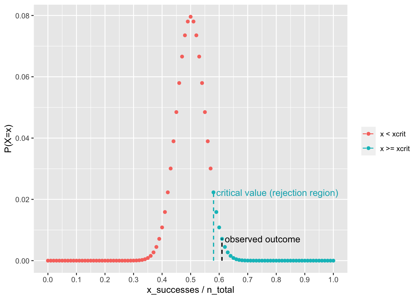
## because of the notes discussed above in step 3The decision rule above can also be expressed in terms of a critical value. The critical value \(\widehat{\theta}_{\text{crit}}\) in NHST is the outcome such that \(P(\widehat{\theta} \geq \widehat{\theta}_{\text{crit}} | H_0) \leq \alpha\).
As such, any observed outcome equal to the critical value or more extreme than the critical value will lead to the rejection of the null. For this reason, values more extreme than the critical value are said reside in the rejection region.
To obtain critical values, we need to get an outcome that
corresponds to a specific probability. This is given to us
by the qbinom() function, again with lower.tail=FALSE.
n <- 100
p <- 0.5
xcrit <- qbinom(0.05, n, p, lower.tail=FALSE)

## Have to divide by n because we are working with
## proportions not counts
phatcrit <- xcrit / n

xcrit
## [1] 58## [1] 0.58
The five steps outlined above are the core of
null-hypothesis significance testing, and working through
each step in the longhand format that we just did is
important to be able to do. This is because these five steps
are completely general and will perfectly apply to any
situation you might find yourself in. That said, in many
situations, R has built-in functions to handle all five
steps in one line of code. When making inferences from a
binomial distribution, you can use the binom.test()
function.
xobs <- 61       ## number of observed successes
n <- 100         ## n parameter of H0
p <- 0.5         ## p parameter of H0
alpha <- 0.05    ## error rate tolerance
alt <- 'greater' ## test direction

## Use built in `binom.test()`
binom.test(xobs,
           n,
           p,
           alternative = alt,
           conf.level = 1 - alpha
           )
##
## Exact binomial test
##
## data: xobs and n
## number of successes = 61, number of trials = 100, p-value = 0.0176
## alternative hypothesis: true probability of success is greater than 0.5
## 95 percent confidence interval:
## 0.5230939 1.0000000
## sample estimates:
## probability of success
## 0.61