8 Moments of a random variable
Sometimes specififying the entire probability distribution is cumbersome or unnecessary. In these cases, we sometimes seek to characterize the shape of the distribution using the moments of the random variable. The moments of a random variable are simple scalar values that are computed from knowledge of the probability distribution. Moments provide insiight into a probability distribition’s central tendency, dispersion, skewness, kurtosis, etc.
8.1 The expected value of a random variable
It’s cool to know that moments are a thing but a full treatment of moments is beyond the scope of this book. It will be sufficient to know that the first moment of a random variable is the expected value of the random variable and the second moment is the variance of the random variable.
The expected value of a random variable is a measure of the central tendency of the random variable. It is also called the population mean. The expected value of a random variable is a statement of where most of your data is likely to fall if you sample the random variable many times. It is defined as the weighted average of the possible outcomes of the random variable, where the weights are given by the probability of each outcome.
For a discrete random variable, the expected value is given by the following equation:
\[\begin{align} \mathbb{E}\big[X\big] &= \mu \\ &= x_1 p(x_1) + x_2 p(x_2) + \ldots + x_n p(x_n) \\ &= \sum_{i}^{n} x_i p(x_i) \end{align}\]
When dealing with continuous random variables, this equation becomes the following:
\[\begin{align} \mathbb{E}\big[X\big] &= \mu \\ &= \int_{a}^{b} f(x) dx \end{align}\]
where the possible outcomes of the random variable \(X\) are continuous in the interval \([a, b]\), and \(f(x)\) is the probability density function of \(X\).
8.2 The variance of a random variable
We saw that for discrete random variables, population variance is defined as the expected squared deviation from the mean, as given by the following equation:
The variance of a random variable – called the population variance is a measure of the spread of the random variable. It is a statement of how much the data is likely to deviate from the expected value if you sample the random variable many times. It is defined as the expected value of the squared deviation of the random variable from its mean.
For discrete random variables, the variance is given by the following equation:
\[\begin{align} \mathbb{Var}\big[X\big] &= \sigma^2 \\ &= E((X - \mu)^2) \\ &= \sum_i x_{i}^2 p(X=x_{i}) - \mu^2 \end{align}\]
For continuous random variables, this equation becomes the following:
\[\begin{align} \mathbb{Var}\big[X\big] &= \sigma^2 \\ &= E((X - \mu)^2) \\ &= \int_{a}^{b} (x - \mu)^2 f(x) dx \end{align}\]
Computing the expected value and the variance of a continuous random variable requires the evauluation of integrals. This book will not cover the details of how to compute these integrals. Instead, it will be sufficient to know that the integral of a function over a given interval is the area under the curve of the function over that interval. That will be more than enough for our purposes.
8.3 Using sample statistics to estimate random variable moments
8.3.1 Population mean for discrete \(X\)
Let \(X\) be a discrete random variable.
Let \(\boldsymbol{x} = \{x_1, \ldots, x_n\}\) be a sample from \(X\).
The central tendency of the sample \(\boldsymbol{x}\) is given by the sample mean \(\bar{\boldsymbol{x}}\): \[ \begin{align} \bar{\boldsymbol{x}} &= \frac{1}{n} \sum_{i=1}^{n} x_{i} \end{align} \]
The true central tendency of \(X\) is given by the population mean which is denoted by \(\mu\) and is defined by an operation called the expected value of \(X\) denoted \(\mathbb{E}\big[X\big]\):
\[ \begin{align} \mathbb{E}\big[\boldsymbol{X}\big] &= \mu \\ &= x_1 p(x_1) + x_2 p(x_2) + \ldots + x_n p(x_n) \\ &= \sum_{i}^{n} x_i p(x_i)\\ \end{align} \]
If we do not know the true value of the population mean \(\mu\) then we can estimate it using the sample mean \(\bar{\boldsymbol{x}}\). \[ \begin{align} \hat{\mu} &= \bar{\boldsymbol{x}} \end{align} \]
This is called a point estimate of \(\mu\), because we are specifying a single number (i.e., a single point) that is our best guess for its true value. Later, we will learn about interval estimates of population parameters, which provide a range of best guess (e.g., we might try to say that we are \(95\%\) percent sure that the true value of some population parameter is between some lower value and some upper value). We will see how to generate interval estimates in a later lecture. For now, it is sufficient to understand their conceptual relationship to point estimates.
8.3.2 Population variance for discrete \(X\)
Similarly, a common measure of the spread of a sample is given by the sample variance \(\boldsymbol{s}^2\):
\[ \begin{align} \boldsymbol{s}^2 &= \frac{1}{n-1} \sum_{i=1}^{n} (x_i - \bar{\boldsymbol{x}})^2 \end{align} \]
The true variance of \(X\) is given by the population variance which is denoted by \(\sigma^2\) and is defined as follows: \[ \begin{align} \mathbb{Var}\big[\boldsymbol{X}\big] &= \sigma^2 \\ &= \mathbb{E}\big[(X - \mu)^2\big] \\ &= \sum(x^2 - 2x\mu + \mu^2) p(x) \\ &= \sum x^2 p(x) - \sum 2 x \mu p(x) + \sum \mu^2 p(x) \\ &= \sum x^2 p(x) - 2 \mu \sum x p(x) + \mu^2 \sum p(x) \\ &= \sum x^2 p(x) - 2 \mu^2 + \mu^2 \\ &= \left(\sum_i x_{i}^2 p(x_{i})\right) - \mu^2 \end{align} \]
If we do not know the true value of the population variance \(\sigma^2\) then we can estimate it using the sample variance \(\bar{\boldsymbol{s}^2}\). \[ \begin{align} \hat{\sigma^2} &= \boldsymbol{s}^2 \\ \end{align} \]
8.3.3 Discrete \(X\) example
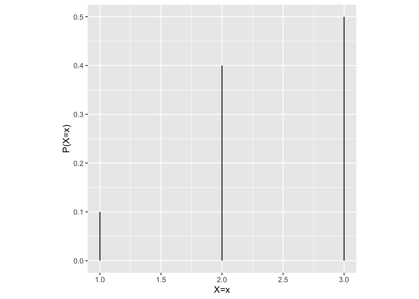
As a concrete example, consider the following discrete probability distribution corresponding to the random variable \(X\).

Since we are explicitly given the probability distribution — i.e., we are told exactly what the probability of each event is — so we can calculate the population mean \(\mu\) as follows:
\[ \begin{align} \mu &= \mathbb{E}\big[\boldsymbol{X}\big] \\ &= \sum_{i}^{n} x_i p(x_i) \\ &= (1 \times 0.1) + (2.0 \times 0.4) + (3.0 \times 0.5) \\ &= 2.4 \end{align} \]
Now suppose that we draw a the following sample of \(n=10\) from this distribution:
## [1] "x:"## [1] 2 2 3 3 3 2 3 3 3 1## [1] "sample mean:"## [1] 2.5The sample mean of this sample is \(\bar{\boldsymbol{x}} =\) 2.5. Note that our sample mean is not equal to the population mean (it’s just a fluke if it is). In fact, every time we run this experiment, we will likely get a different sample mean. Lets run it 5 more times and check each one.
## [1] "x:"
##  [1] 3 2 3 3 3 2 3 1 3 3
## [1] "sample mean:"
## [1] 2.6
## [1] "x:"
##  [1] 2 2 2 3 1 3 3 2 1 2
## [1] "sample mean:"
## [1] 2.1
## [1] "x:"
##  [1] 2 3 3 2 3 1 3 3 3 2
## [1] "sample mean:"
## [1] 2.5
## [1] "x:"
##  [1] 2 2 3 1 1 3 3 3 2 3
## [1] "sample mean:"
## [1] 2.3
## [1] "x:"
##  [1] 1 3 2 2 3 1 3 2 3 1
## [1] "sample mean:"
## [1] 2.18.3.4 Population mean and variance for continuous \(X\)
Let \(X\) be a continuous random variable.
Let \(\boldsymbol{x} = \{x_1, \ldots, x_n\}\) be a sample from \(X\).
Sample statistics are computed in exacrtly the same way regardless of whether \(X\) is continuous or discrete.
Population parameters are again computed in terms of the expected value operator, but the way this operator works is a bit different depending on whether \(X\) is continuous or discrete.
In particular, if \(X\) is continuous, then we will replace discrete sums (i.e., \(\sum x\)) with continuous integrals (i.e., \(\int x dx\)).
8.3.4.1 Continuous \(X\) mean
\[ \begin{align} \bar{\boldsymbol{x}} &= \frac{1}{n} \sum_{i=1}^{n} x_{i} \\ \mathbb{E}\big[\boldsymbol{X}\big] &= \mu \\ &= \int x f(x) dx \\ \\ \hat{\mu} &= \bar{\boldsymbol{x}} \end{align} \]
8.3.4.2 Continuous \(X\) variance
\[ \begin{align} \boldsymbol{s}^2 &= \frac{1}{n-1} \sum_{i=1}^{n} (x_i - \bar{\boldsymbol{x}})^2 \\ \mathbb{Var}\big[\boldsymbol{X}\big] &= \sigma^2 \\ &= \mathbb{E}\big[(X - \mu)^2\big] \\ &= \int(x^2 - 2x\mu + \mu^2) f(x) dx \\ &= \int x^2 f(x) dx - \int 2 x \mu f(x) dx + \int \mu^2 f(x) dx \\ &= \int x^2 f(x) dx - 2 \mu \int x f(x) dx + \mu^2 \int f(x) dx \\ &= \int x^2 f(x) dx - 2 \mu^2 + \mu^2 \\ &= \left(\int x^2 fx \right) - \mu^2 \\ \hat{\sigma^2} &= \boldsymbol{s}^2 \\ \end{align} \]
8.3.5 Continuous \(X\) example
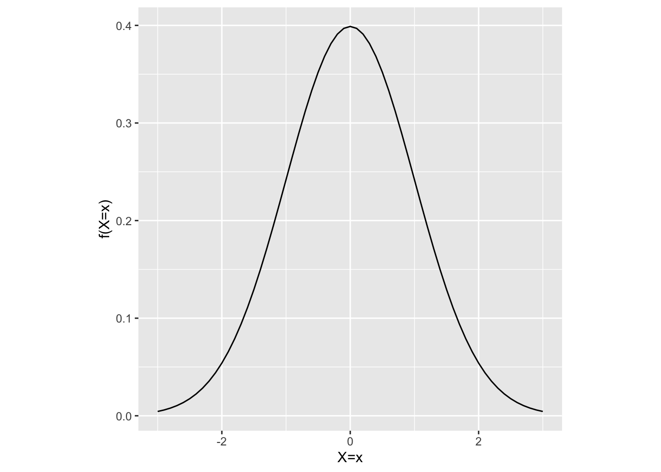
As a concrete example, consider the following continuous probability distribution corresponding to the random variable \(X\).

As for our discrete \(X\) example, we are explicitly given the probability distribution — i.e., we are told exactly what the probability density of each event is — so we can calculate the population mean \(\mu\) as follows:
\[ \begin{align} \mu &= E(\boldsymbol{X}) \\ &= \int x p(x) dx \\ &= 0 \\ \end{align} \]
Now suppose that we draw a the following sample of \(n=10\) from this distribution:
## [1] "x:"## [1] 0.2885703 -1.6685417 0.8510622 0.2157761 -1.8147071 -0.1734513
## [7] 0.9537678 0.7037876 -0.6312850 0.9075918## [1] "sample mean:"## [1] -0.03674294The sample mean of this sample is \(\bar{\boldsymbol{x}} =\) -0.0367429. As for our discrete \(X\) exmaple, we see that our sample mean is not equal to the population mean. Lets run it 5 more times to demonstrate again that the sample mean is indeed a ranomd variable.
## [1] "x:"
##  [1] -0.3969633  0.3819590  0.9285327  0.3905761 -0.6527025  0.8199824
##  [7]  1.4774301 -0.9291964 -0.1821943  1.0036585
## [1] "sample mean:"
## [1] 0.2841082
## [1] "x:"
##  [1] -0.85199189 -1.71937580 -0.49469904  1.06648978 -1.36184763 -0.24830383
##  [7]  0.96193008  0.04692745  0.56691905  1.62398016
## [1] "sample mean:"
## [1] -0.04099717
## [1] "x:"
##  [1]  0.90077121  0.59119065  0.49098641 -1.15841660  0.83919689  0.54210662
##  [7]  0.40362073  0.05720034 -1.27104788  0.15359375
## [1] "sample mean:"
## [1] 0.1549202
## [1] "x:"
##  [1]  1.25495610 -0.61171296 -1.80084925  1.83802787 -0.56427794  1.14035660
##  [7]  0.62405347  1.65773610 -0.04209058 -0.30044453
## [1] "sample mean:"
## [1] 0.3195755
## [1] "x:"
##  [1]  1.7322580  2.1565298  0.3185189  0.1698470  0.7423495 -0.6725367
##  [7]  0.4978262 -0.9896120 -0.2974796  0.7948835
## [1] "sample mean:"
## [1] 0.4452585