16 Inferential error and statistical power
16.1 Type I versus Type II errors
16.1.1 Definitions
Hypothesis testing is about using noisy data to make decisions about what we think the true state of the universe is.
Sometimes, our procedure for making these decisions will lead us to make the correct decision, but sometimes we will make the wrong decision.
In the context of hypothesis testing, there are two ways to make a correct decision and two ways to make an incorrect decision. These are summarised in the following table.
| H0 True | H1 True | |
|---|---|---|
| Reject H0 | Type I error (\(\alpha\)) | Power (\(1-\beta\)) |
| Fail to reject H0 | Confidence (\(1-\alpha\)) | Type II error (\(\beta\)) |
Here, we have introduced the concept of power.
Power is the probability of correctly rejecting \(H_0\).
Power can only be computed with respect to some fully specified \(H_1\).
This is best seen with a visualisation.
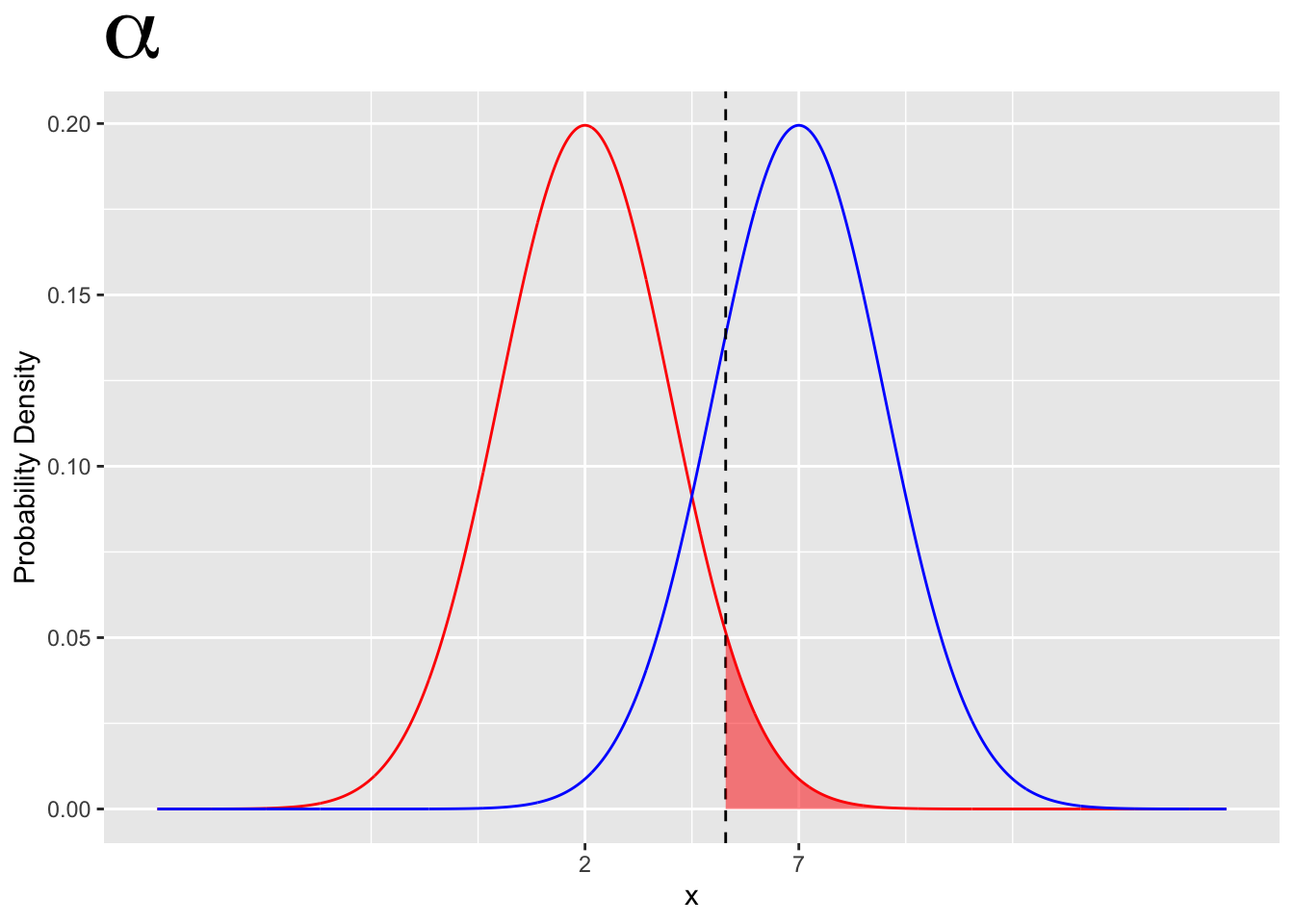
- Type I error is given by \(\alpha\)
- The probability of a type I error is given by the area under the \(H_0\) curve in the rejection region.
- A type I error is the probability of incorrectly rejecting \(H_0\)
- Type I error is completely determined by \(H_0\)
- Type I error does not depend on \(H_1\)

- Power is given by \(1 - \beta\)
- Power is given by the area under the \(H_1\) curve in the rejection region.
- Power can depends on both \(H_0\) and \(H_1\)
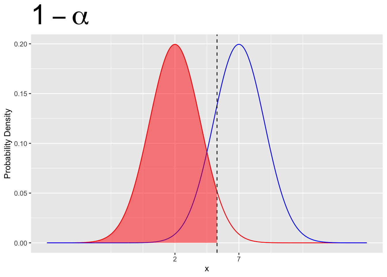
- Confidence is given by \(1 - \alpha\)
- Confidence is given by the area under the \(H_0\) curve outside the rejection region.
- Confidence depends only on \(H_0\)
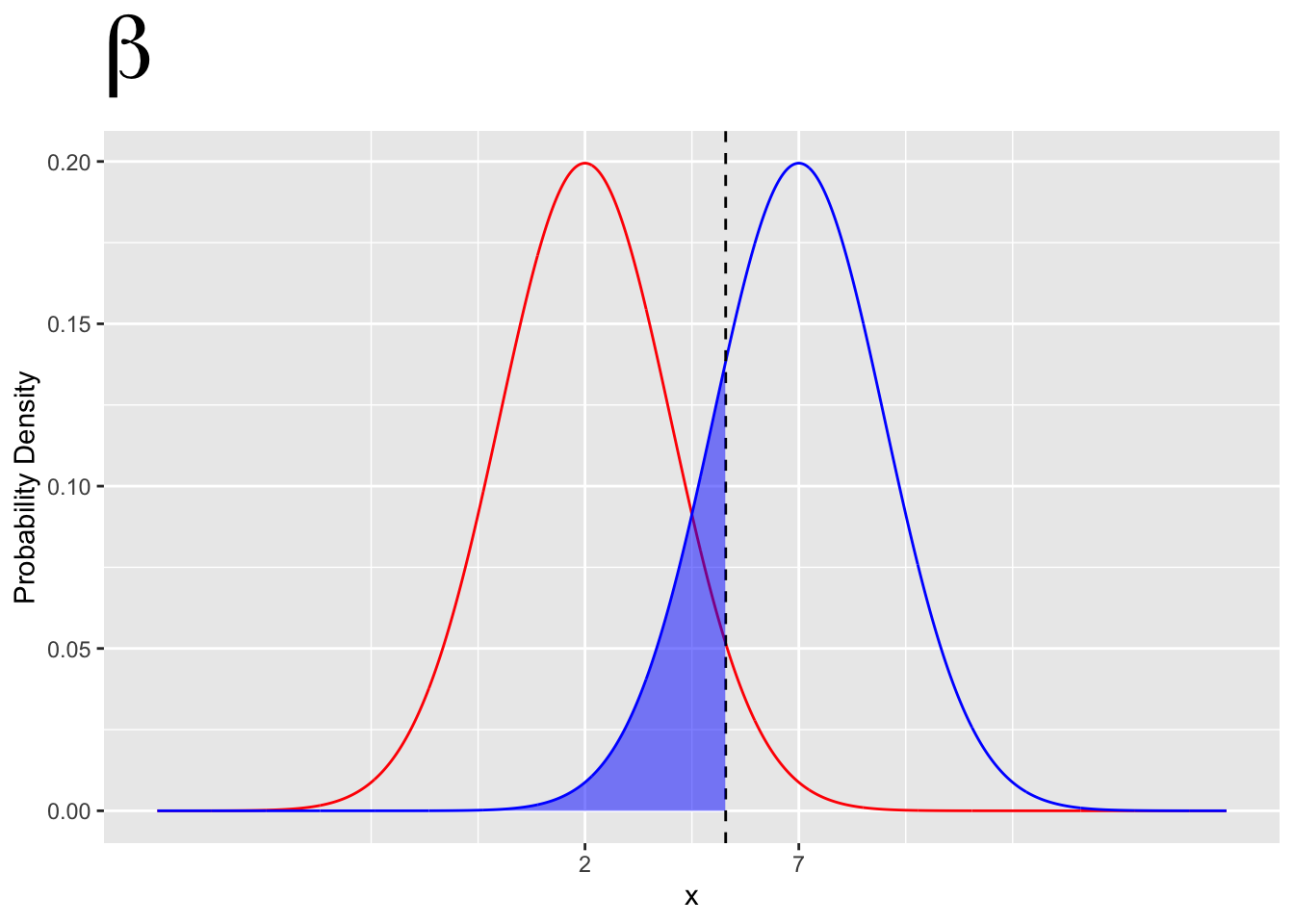
- Type II error is given by \(\beta\)
- The probability of a type II error is given by the area under the \(H_1\) curve outside the rejection region.
- A type II error is the probability of incorrectly failing to reject \(H_0\)
- Type II error depends on both \(H_0\) and \(H1\)
16.2 power
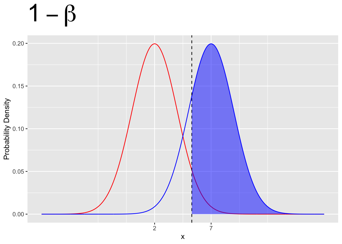
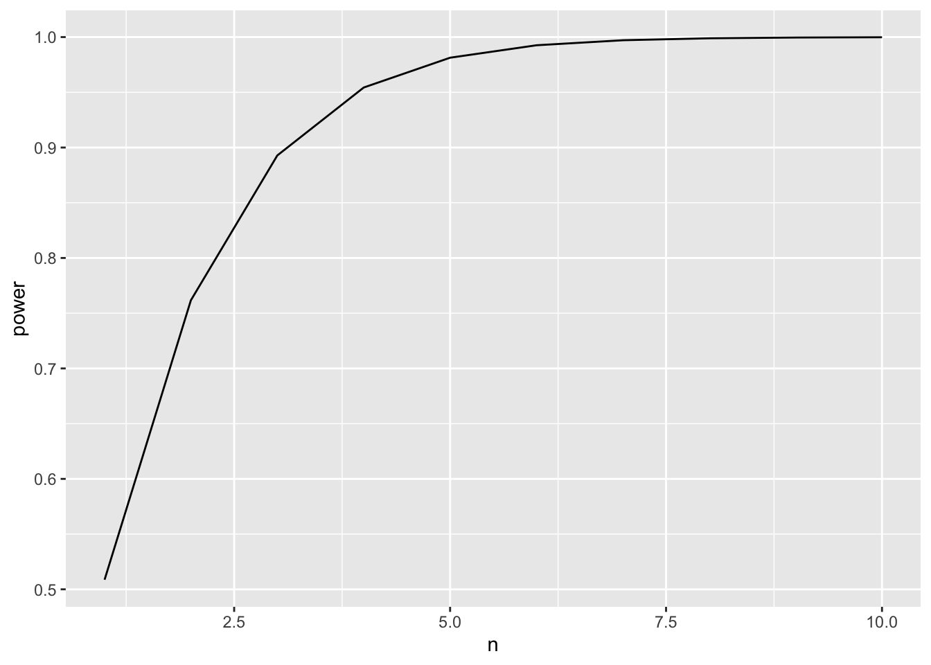
- In general, we want as much power as possible.
- This is because, if \(H_0\) isn’t true, then we’d really like to reject it.
- How can we increase power?
16.2.1 Increase the distance between \(H_0\) and \(H_1\)
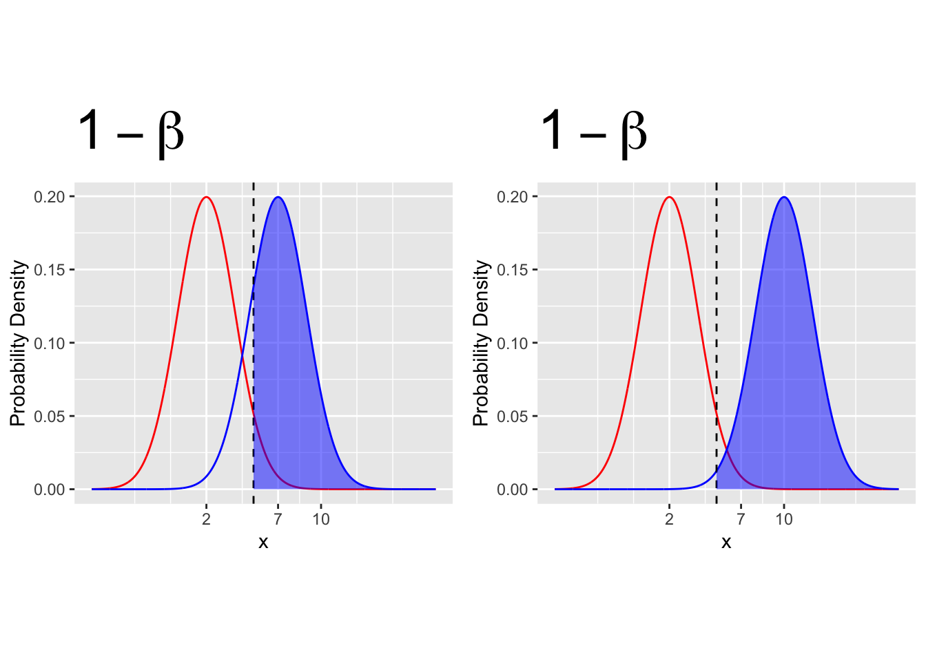
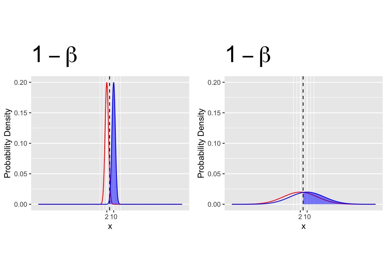
- The closer together the \(H_0\) and \(H_1\) distributions, the less power we have.
