12 Using R to compute probabilities
For most probability distributions, R has 4 built-in functions that tell you almost everything you will ever want to know about them.
For the Binomial distribution, these functions are the following:
dbinom(x): Probability mass functionpbinom(x): Cumulative distribution functionqbinom(p): quantile functionrbinom(n): function for random samples
For the Normal distributions, these functions are the following:
dnorm(x): Probability density functionpnorm(x): Cumulative distribution functionqnorm(p): quantile functionrnorm(n): function for random samples
You can see the naming convention adopted by R right away.
The
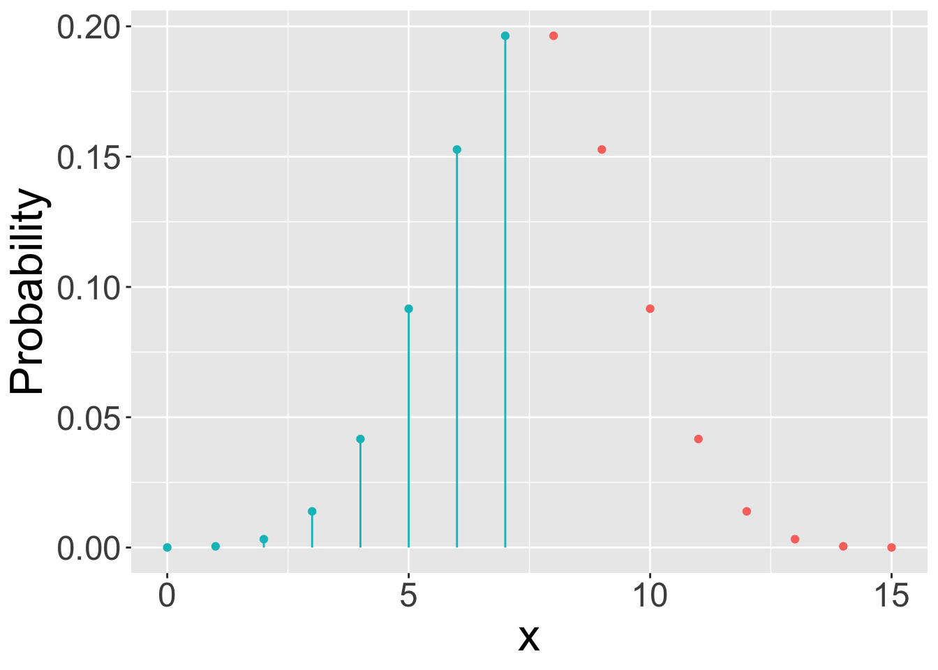
dfunctions are mass or density functions.For discrete distributions, these functions return \(P(X=x)\). E.g.,
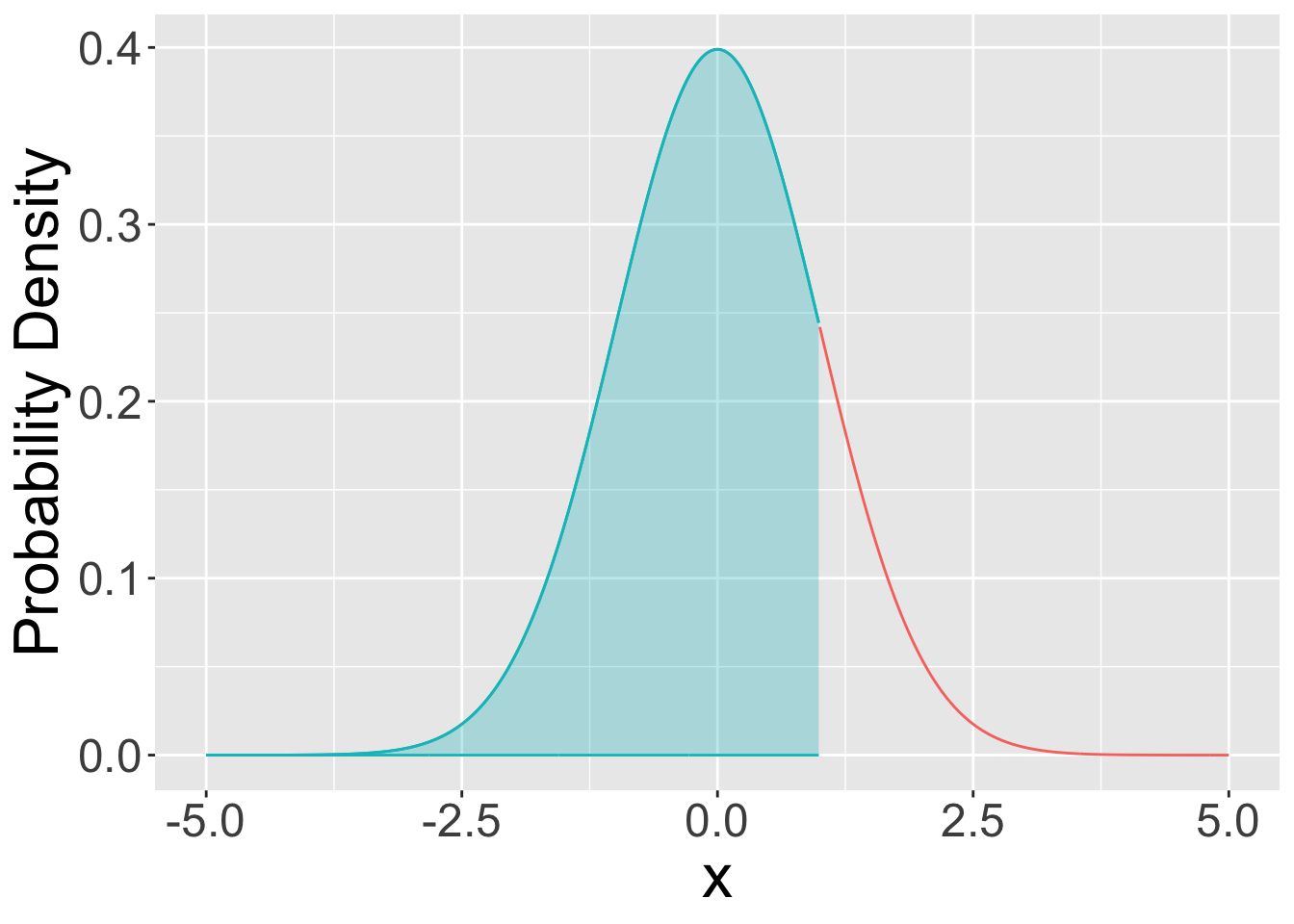
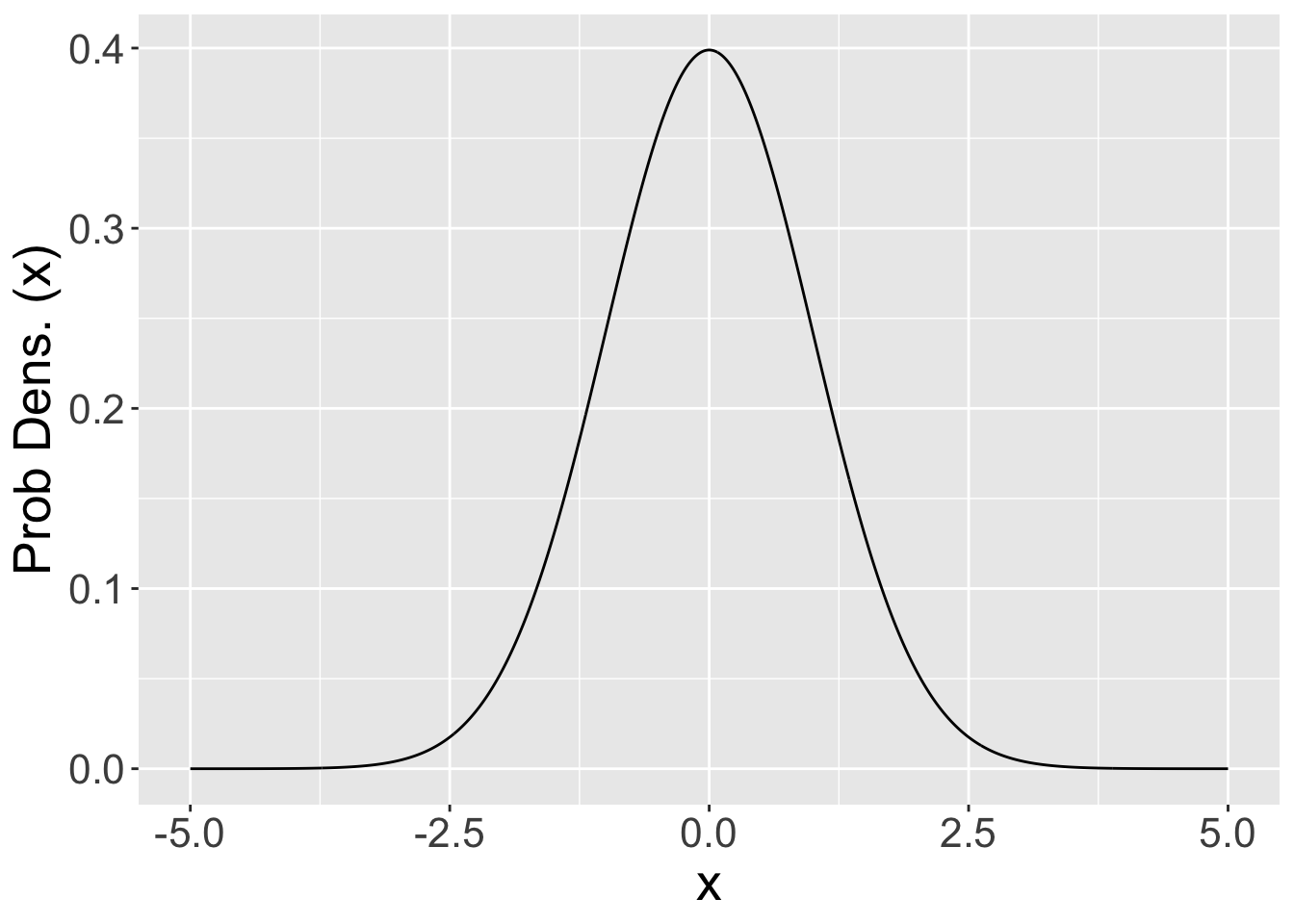
dbinom(x, n, p)returns the probability that a binomial random variable with parameters \(n\) and \(p\) will yield a value of \(x\).For continuous distributions, these functions return a probability density. To get probability, we must consider a range of outcomes \([a, b]\) and compute the area under the curve. Computing the exact area under the curve requires evaluating an integral, which is too hard for us and awkward to do using a
dfunction. It will be best to use apfunction in this case (see below).
The
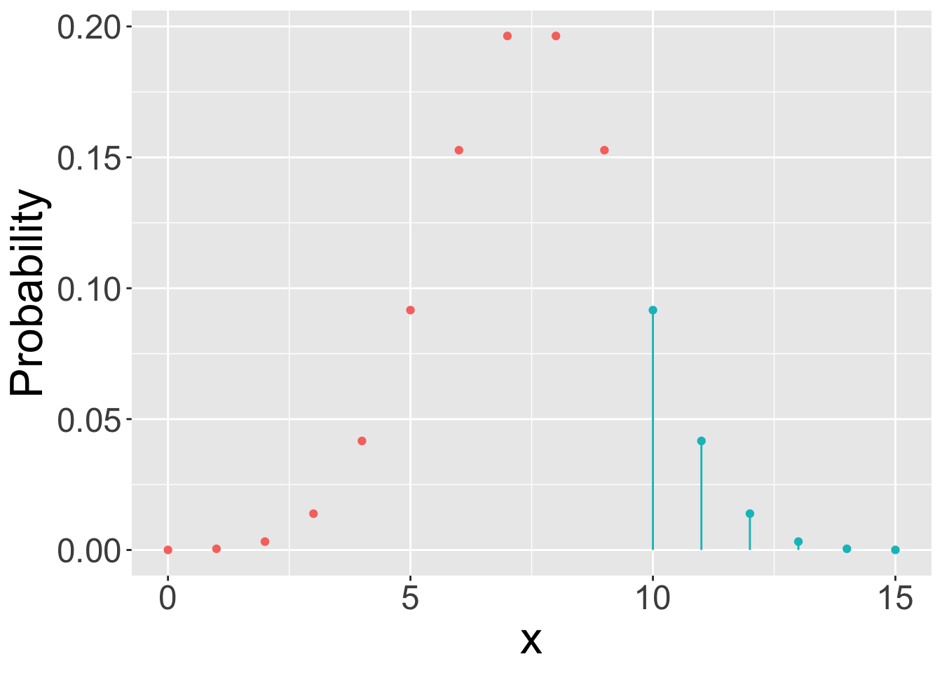
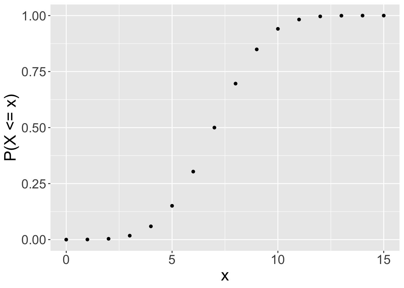
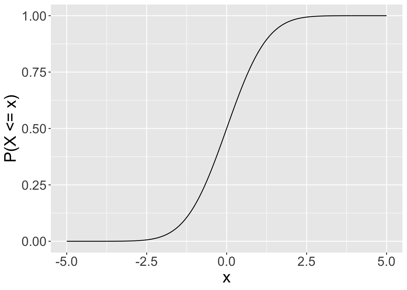
pfunctions are cumulative probability functions.- By default these functions return \(P(X \leq x)\). If you
specify
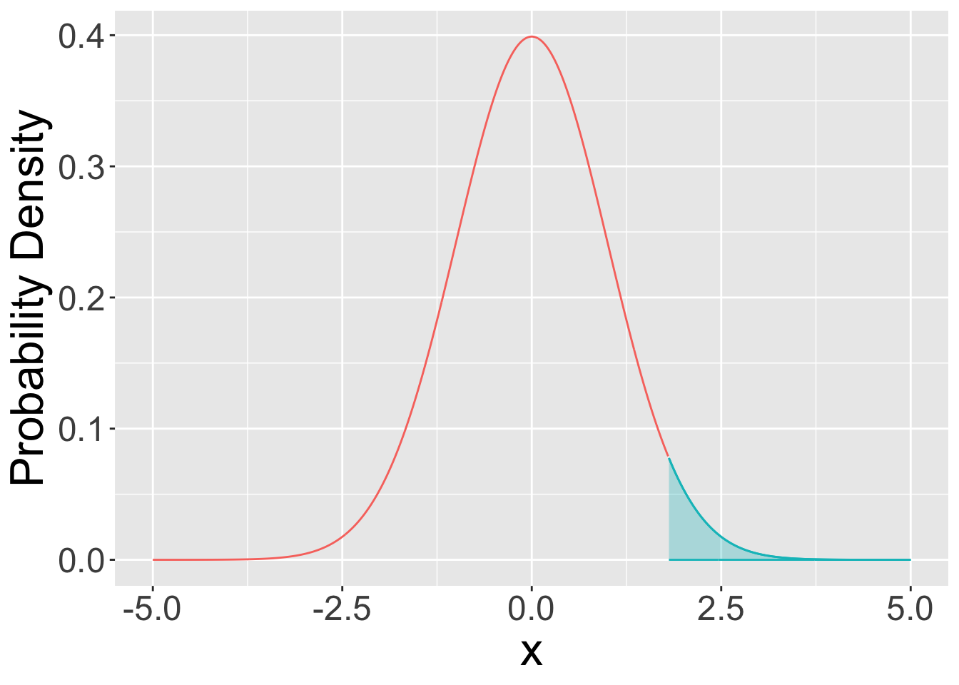
lower.tail=FALSEthen these functions return \(P(X\>x)\). Be careful when using these functions to appreciate that for continuous distributions \(P(X \leq x)=1-P(X \geq x)\) but for discrete distributions \(P(X \leq x)=1-P(X \geq x+1)\). All that is basically just to say be careful when considering whether to use greater than or greather than and equal to etc.
- By default these functions return \(P(X \leq x)\). If you
specify
The
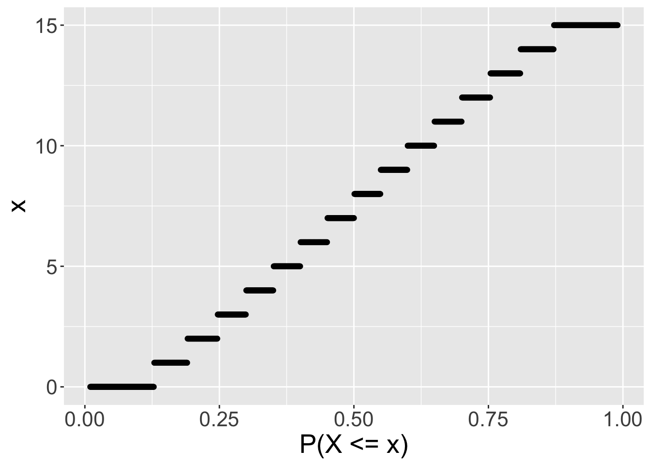
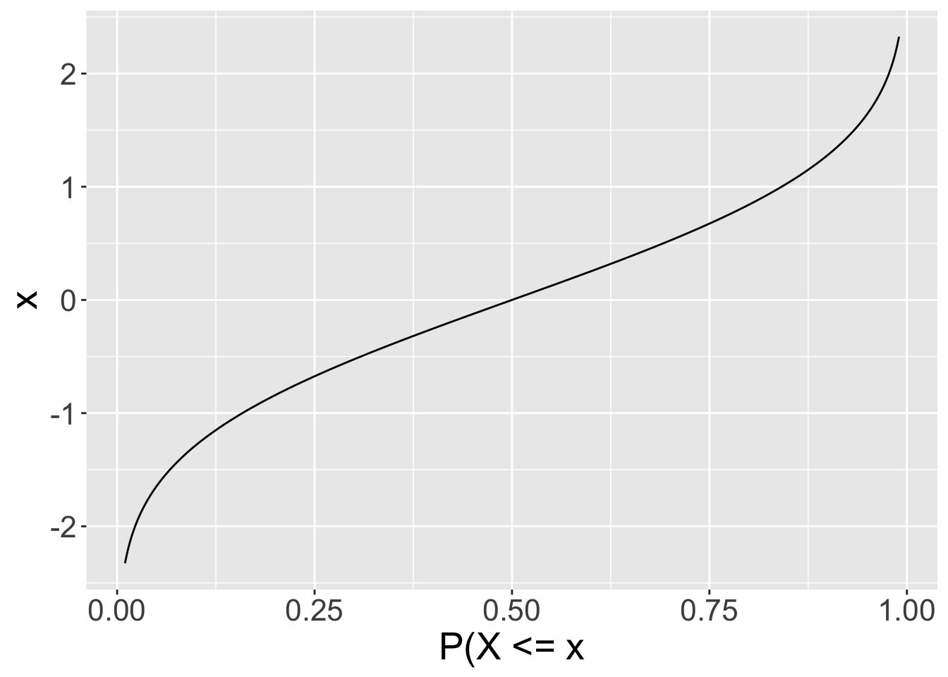
qfunctions are quantile functions.- They are the inverse of the cumulative probability functions. Here, you specify a cumulative probability \(q\), and the function returns the value of \(x\) such that \(P(X\<x)=q\).
The
rfunctions generate random samples.
pmf: probabilities are given by values on the y-axis.

cdf: cumulative probabilities \((X\<x)\) are given by reading values on the y-axis.
qf: use this function to specify a probability (x-axis) and get the value that satisfies this probability from the y-axis.
pdf: probabilities are given by the area under the curve.
cdf: cumulative probabilities \((X\<x)\) are given by reading values on the y-axis.
qf: use this function to specify a probability (x-axis) and get the value that satisfies this probability from the y-axis.
In general, I think it is important for you to be able to read each of the types of plots above, so please really try to encode these and think about them deeply.