17 Confidence intervals
17.1 Confidence intervals for two-tailed tests
Way back in the beginning of the class we covered descriptive statistics, and more recently we have used some of these descriptive statistics as estimates of population parameters.
For example, we have used the sample mean \(\bar{x}\) as an estimate of the population mean \(\mu_X\).
This is an example of a point estimate of a population parameter, and it represents our single best guess about the true value of the parameter in question.
An alternative approach to point estimation is to instead try to estimate a range of values in which the true value of the parameter is likely to reside.
This is called interval estimation and it is accomplished by constructing a confidence interval.
It is simplest to conceive of confidence intervals in the context of two-tailed tests, so what follows is for that situation.
To construct a confidence interval for the population mean \(\mu_X\) (assuming the population variance \(\sigma_X^2\) is known), first compute the sample mean \(\bar{x}\).
Next, the width of the CI is the same as the width of the distribution of sample means required to cover \(1-\alpha\) percent of it’s probability. Call this width \(w\).
Then the confidence interval estimate of \(\mu_X\) is given by \(CI = \left[ \bar{x}-\frac{w}{2} \text{, } \bar{x}+\frac{w}{2} \right]\)

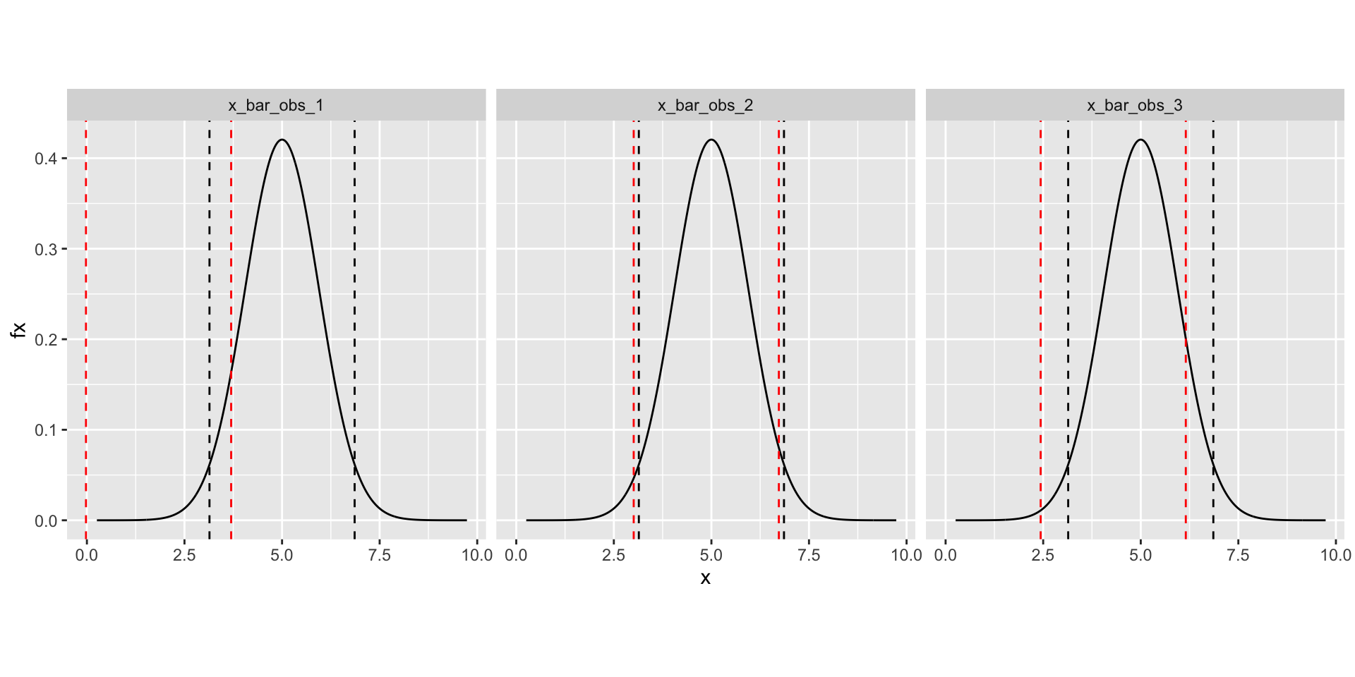
In the above plot, red vertical lines mark the confidence interval and black vertical lines mark the critical values.
CI is always centred around the observed value.
Critical values are always centred around the mean of the null sampling distribution.
This can all be written concisely as follows:
\[ CI_{1-\alpha} = \left[ \bar{x} - \Phi_{\bar{X}}^{-1}(1-\frac{\alpha}{2}), \text{ } \bar{x} + \Phi_{\bar{X}}^{-1}(1-\frac{\alpha}{2}) \right] \]
- For example, the 95% confidence interval for the population mean of \(X \sim N(\mu_X, \sigma_X)\) is given by:
\[\begin{align} CI_{1-0.05} &= \left[ \bar{x} - \Phi_{X}^{-1}(1-\frac{0.05}{2}), \text{ } \bar{x} + \Phi_{X}^{-1}(1-\frac{0.05}{2}) \right] \\ \\ CI_{.95} &= \left[ \bar{x} - \Phi_{X}^{-1}(1-0.025), \text{ } \bar{x} + \Phi_{X}^{-1}(1-0.025) \right] \\ \\ &= \left[ \bar{x} - \Phi_{X}^{-1}(0.975), \text{ } \bar{x} + \Phi_{X}^{-1}(0.975) \right] \end{align}\]
Notice that just like the point estimate \(\bar{x}\), a confidence interval is also a random variable, and so changes with every experiment performed.
We can demonstrate this by repeating the procedure and observing that the obtained confidence intervals are different with each repetition.

Common misconceptions about confidence intervals:
There is a 95% chance that the true population mean falls within the confidence interval.
The mean will fall within the confidence interval 95% of the time.
Neither of these statements is true. Rather, a 95% level of confidence means that 95% of the confidence intervals calculated from a set of random samples will contain the true population mean. For example, if you repeated your study 100 times, we would expect that 95 out of 100 of these studies to produce confidence intervals that contain the true population mean.
17.2 Confidence intervals for one-tailed tests
In the context of a one-tailed test, confidence intervals always take the form \((a, \infty)\) for a greater than test direction or \((\infty, a)\) for a less than test direction.
This is like saying that with a greater than test we really only care about a lower bound on the interval beyond which we would reject the null.
A similar logic holds for less than tests.
To compute \(a\) we follow much the same procedure as with two-tailed tests, but since it’s a one-tailed test, we use all of \(\alpha\) when computing the finite boundary.
CI for greater than:
\[ CI_{1-\alpha} = \left[ \bar{x} - \Phi_{\bar{X}}^{-1}(1-\alpha), \text{ } \infty \right] \]
- CI for less than:
\[ CI_{1-\alpha} = \left[ \infty, \text{ } \bar{x} - \Phi_{\bar{X}}^{-1}(1-\alpha) \right] \]