3 Introduction to calculus
3.1 Derivatives
A derivative represents the rate at which a function is changing at any point. For example, if you consider the distance traveled over time, the derivative of this distance with respect to time gives you the speed. Let’s use Python to visualize a simple function and its derivative to understand how it represents change.
import numpy as np
import matplotlib.pyplot as plt

# Define the function and its derivative
def f(x):
    return x**2

def df_dx(x):
    return 2*x

# Generate x values
x = np.linspace(-10, 10, 400)

# Plot the function and its derivative
plt.figure(figsize=(10, 6))
plt.plot(x, f(x), label='f(x) = x^2')
plt.plot(x, df_dx(x), label="f'(x) = 2x", linestyle='--')
plt.title('Function and its Derivative')
plt.xlabel('x')
plt.ylabel('y')
plt.legend()
plt.grid(True)
plt.show()
3.1.1 Practive with derivatives
Consider the function \(f(x) = x^3 - 3x^2 + x\). Follow the steps below to explore its derivative.
Sketch the Function: On graph paper or using a graphing software, plot the function \(f(x) = x^3 - 3x^2 + x\) for \(x\) values ranging from -2 to 4. Describe the behavior of the function based on your graph.
Predict the Derivative: Before calculating the derivative, discuss in your group where you think the function is increasing, decreasing, or has a flat slope (inflection points). Predict how these observations might reflect on the graph of the derivative.
Calculate the Derivative: Calculate the derivative of the function, \(f'(x)\). \(f'(x) = 3x^2 - 6x + 1\).
Sketch the Derivative: Plot the derivative on the same or a new graph for the same \(x\) values. Compare this graph to the original function’s graph. How does the derivative reflect the behavior of the original function?
3.2 Integrals
An integral calculates the total accumulation of a quantity, such as the total area under a curve. It’s like adding up infinite slices of a quantity to find the whole. Let’s visualize how integrals represent the area under a curve using Python.
def integrate_f(a, b, N=1000):
    x = np.linspace(a, b, N)
    fx = f(x)
    area = np.sum((b-a)/N * fx)
    return area

# Define the limits
a, b = 0, 10

# Calculate the area under the curve
area_under_curve = integrate_f(a, b)

# Visualize
plt.figure(figsize=(10, 6))
plt.fill_between(x, f(x), where=[(i >= a and i <= b) for i in x], color="skyblue", alpha=0.4, label=f'Area = {area_under_curve:.2f}')
plt.plot(x, f(x), label='f(x) = x^2')
plt.title('Area under the curve')
plt.xlabel('x')
plt.ylabel('f(x)')
plt.legend()
plt.grid(True)
plt.show()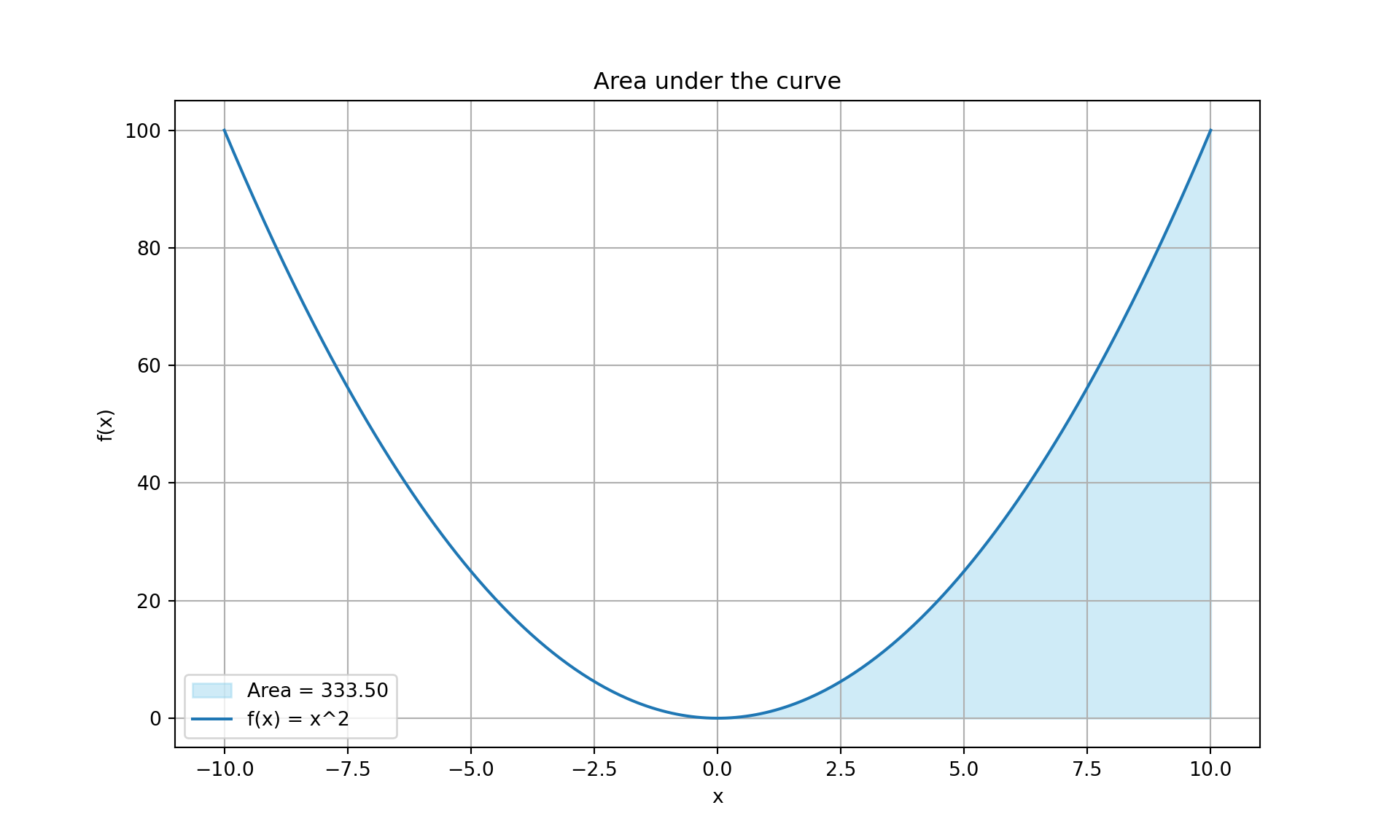
3.2.1 Practice with integrals:
Consider the function \(f(x) = x^2\) as representing some quantity over time.
Sketch the Function: Plot the function \(f(x) = x^2\) for \(x\) values ranging from 0 to 4. This represents the quantity over time.
Estimate the Area: Without performing actual integration, estimate the area under the curve from \(x = 0\) to \(x = 4\). You can do this by dividing the area into shapes (like rectangles or trapezoids) whose area you can easily calculate.
Calculate the Area: Now, calculate the integral of \(f(x)\) from 0 to 4 to find the exact area under the curve. \(\int_{0}^{4} x^2 dx = \frac{1}{3}x^3 \Big|_0^4 = \frac{64}{3}\).
Compare and Discuss: Compare your estimated area with the calculated area. Discuss the differences and why they might exist. What does this area represent in the context of the quantity over time?
Real-World Application: Think of a real-world scenario in neuroscience where calculating the total amount of a quantity over time (like neurotransmitter release) is crucial. Discuss how you would set up the integral to calculate this total amount.