6 Hodgkin-Huxley neuron model
6.1 neuron_func_1
def neuron_func_1():
    '''
    NOTE: dvdt = I - g * (v - E)
    - has stable eq at E
    - looks reasonable for sub threshold dynamics
    - nothing like an action potential
    '''
    tau = 0.01
    T = 100
    t = np.arange(0, T, tau)
    n = t.shape[0]

    I = np.zeros(n)
    v = np.zeros(n)

    vr = -65.0
    E = -65.0
    g = 1.0
    C = 1.0

    v[0] = vr
    I[n // 5:2 * n // 5] = 30.0
    I[3 * n // 5:4 * n // 5] = -30.0

    for i in range(1, n):
        delta_t = t[i] - t[i - 1]
        dvdt = (I[i - 1] - g * (v[i - 1] - E)) / C
        v[i] = v[i - 1] + dvdt * delta_t

    fig, ax = plt.subplots(3, 1, squeeze=False)
    ax[0, 0].plot(t, I, label='I')
    ax[1, 0].plot(t, g * (v - E), label='g * (v - E)')
    ax[2, 0].plot(t, v, label='v')
    [x.legend() for x in ax.flatten()]
    plt.tight_layout()
    plt.show()

neuron_func_1()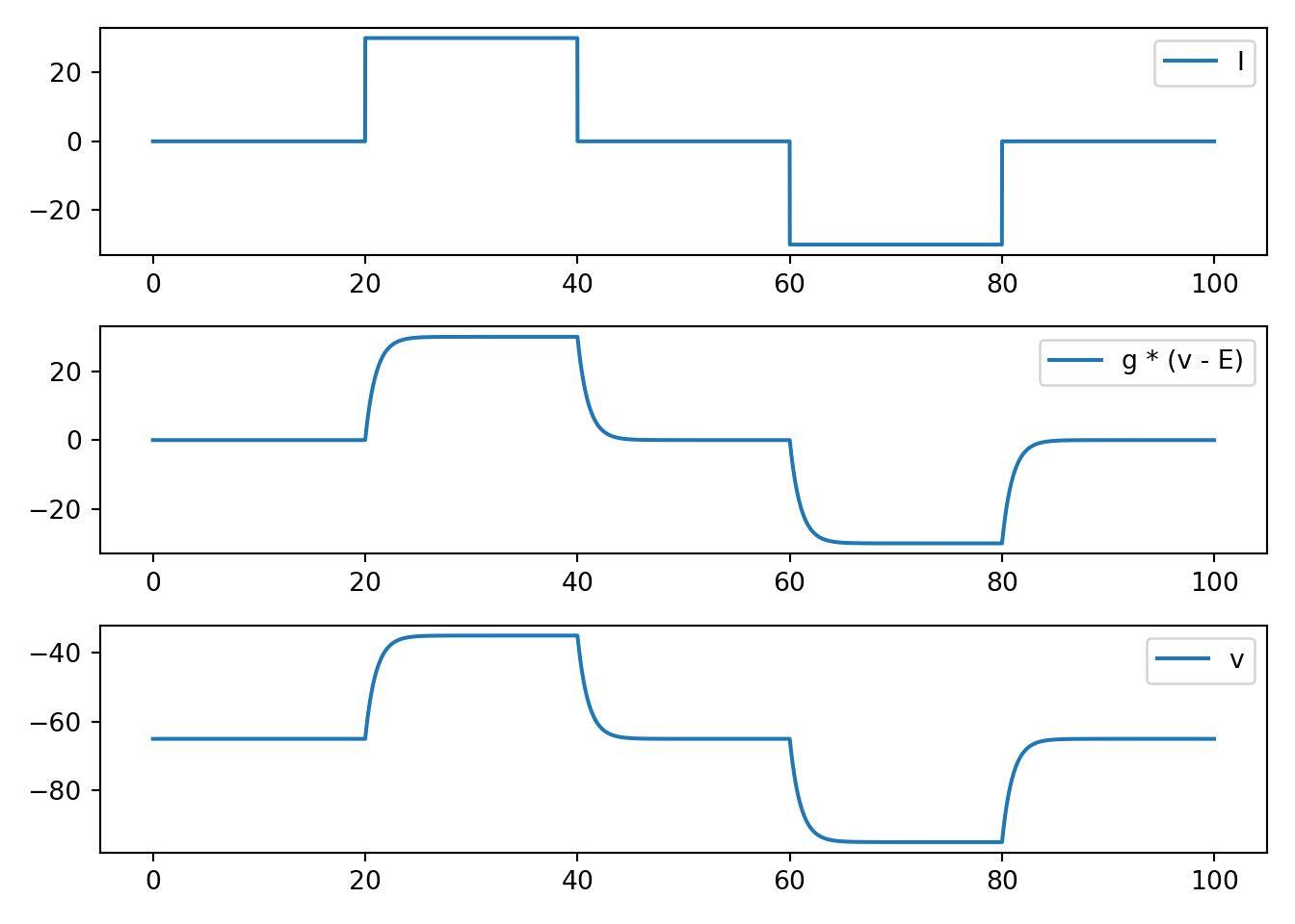
6.2 neuron_func_2
def neuron_func_2():
    '''
    NOTE: dvdt = I - g_a * (v - E_a) - g_b * (v - E_b)
    - has stable eq between E_a and E_b with balance determined by relative g's
    - still looks reasonable for sub threshold
    - still nothing like an action potential
    '''
    tau = 0.01
    T = 100
    t = np.arange(0, T, tau)
    n = t.shape[0]

    I = np.zeros(n)
    v = np.zeros(n)

    vr = -65.0
    E_a = -65.0
    E_b = 65.0
    g_a = 1.0
    g_b = 1.0
    C = 1.0

    v[0] = vr
    I[n // 5:2 * n // 5] = 30.0
    I[3 * n // 5:4 * n // 5] = -30.0

    for i in range(1, n):
        delta_t = t[i] - t[i - 1]
        dvdt = (I[i - 1] - g_a * (v[i - 1] - E_a) - g_b * (v[i - 1] - E_b)) / C
        v[i] = v[i - 1] + dvdt * delta_t

    fig, ax = plt.subplots(3, 1, squeeze=False)
    ax[0, 0].plot(t, I, label='I')
    ax[1, 0].plot(t, g_a * (v - E_a), label='g * (v - E)')
    ax[1, 0].plot(t, g_b * (v - E_b), label='g * (v - E)')
    ax[2, 0].plot(t, v, label='v')
    [x.legend() for x in ax.flatten()]
    plt.tight_layout()
    plt.show()

neuron_func_2()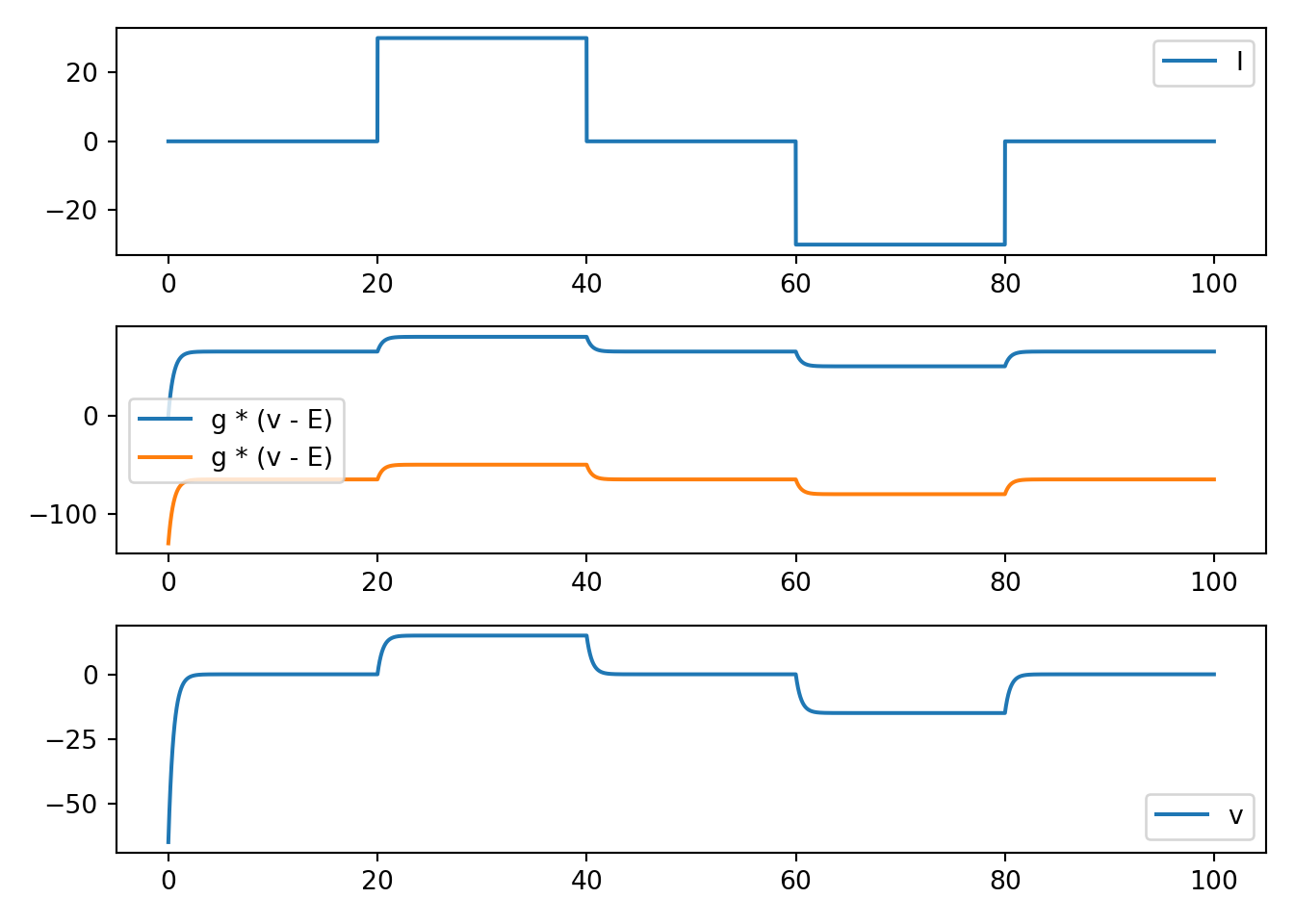
6.3 neuron_func_3
def neuron_func_3():
    '''
    dvdt = I - g_a_max * a * (v - E_a) - g_b * (v - E_b)
    dadt = (a_inf - a) / a_tau
    - Increase due to I can be amplified
    - rise looks an action potential
    - no fall back to rest
    '''

    def g_func_inf(v):
        # sigmoid shape
        return 1 / (1 + 0.1 * np.exp(-0.1 * (v)))

    def g_func_tau(v):
        # bell shape
        mu = -10.0
        sig = 50.0
        return np.exp(-((v - mu) / sig)**2)

    tau = 0.01
    T = 100
    t = np.arange(0, T, tau)
    n = t.shape[0]

    I = np.zeros(n)
    v = np.zeros(n)
    g_a = np.zeros(n)
    g_b = np.zeros(n)

    vr = -65.0

    E_a = -65.0
    E_b = -65.0

    g_a_max = 20.0
    g_b = 1.0

    C = 1.0

    v[0] = vr
    g_a[0] = g_func_inf(vr)

    I[n // 5:2 * n // 5] = 30.0
    I[3 * n // 5:4 * n // 5] = -30.0

    for i in range(1, n):
        delta_t = t[i] - t[i - 1]

        dvdt = (I[i - 1] - g_a_max * g_a[i - 1] * (v[i - 1] - E_a) - g_b *
                (v[i - 1] - E_b)) / C
        dgdt = (g_func_inf(v[i - 1]) - g_a[i - 1]) / g_func_tau(v[i - 1])

        v[i] = v[i - 1] + dvdt * delta_t
        g_a[i] = g_a[i - 1] + dgdt * delta_t

    fig, ax = plt.subplots(5, 1, squeeze=False)
    x = np.arange(-90, 90, 0.01)
    ax[0, 0].plot(x, g_func_inf(x), label='g_func_inf')
    ax[1, 0].plot(x, g_func_tau(x), label='g_func_tau')
    ax[2, 0].plot(t, I, label='I')
    ax[3, 0].plot(t,
                  g_a_max * g_a * (v - E_a),
                  label='g_max * g_a * (v - E_a)')
    ax[3, 0].plot(t, g_b * (v - E_b), label='g_b * (v - E_b)')
    ax[4, 0].plot(t, v, label='v')
    [x.legend() for x in ax.flatten()]
    plt.tight_layout()
    plt.show()

neuron_func_3()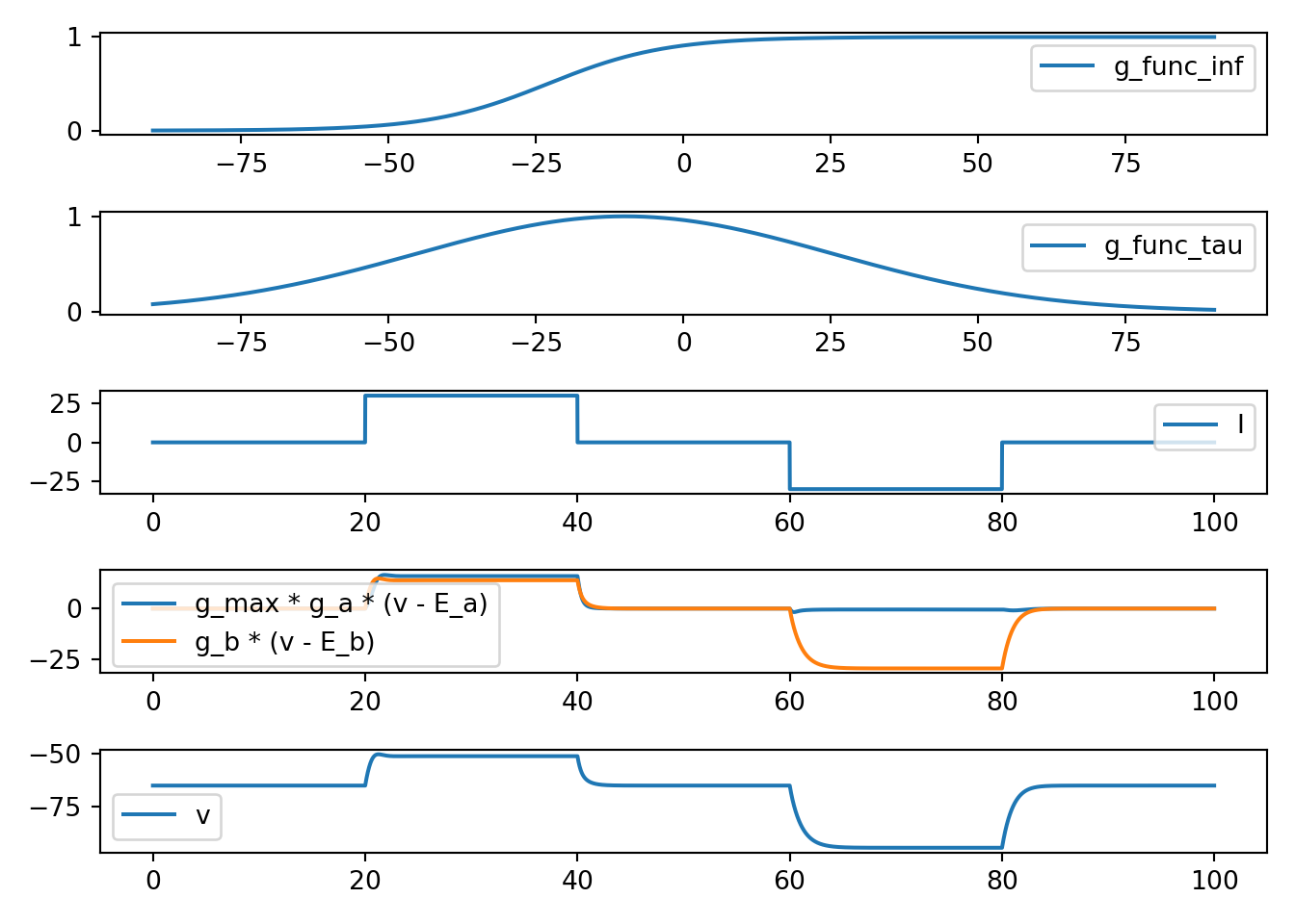
6.4 neuron_func_4
def neuron_func_4():
    '''
    dvdt = I - g_a_max * a * (v - E_a) - g_b_max * b * (v - E_b)
    dadt = (a_inf - a) / a_tau
    dbdt = (b_inf - b) / b_tau
    - Increase due to I can be amplified
    - rise looks an action potential (due to a)
    - can get a fall back to E_b (due to b)
    - fall occurs too slowly to be a normal action potential
    '''

    def g_func_inf_a(v):
        # sigmoid shape
        return 1 / (1 + 0.1 * np.exp(-0.1 * (v)))

    def g_func_inf_b(v):
        # sigmoid shape
        return -1 / (1.1 + 0.1 * np.exp(-0.1 * (v))) + 1

    def g_func_tau_a(v):
        # bell shape
        mu = -10.0
        sig = 60.0
        return (300 / sig) * np.exp(-((v - mu) / sig)**2)

    def g_func_tau_b(v):
        # bell shape
        mu = -10.0
        sig = 50.0
        return (300 / sig) * np.exp(-((v - mu) / sig)**2)

    tau = 0.01
    T = 200
    t = np.arange(0, T, tau)
    n = t.shape[0]

    I = np.zeros(n)
    v = np.zeros(n)
    g_a = np.zeros(n)
    g_b = np.zeros(n)

    vr = -65.0

    E_a = 120.0
    E_b = -70.0

    g_a_max = 1.0
    g_b_max = 2.0

    C = 1.0

    v[0] = vr
    g_a[0] = g_func_inf_a(vr)
    g_b[0] = g_func_inf_b(vr)

    I[n // 5:2 * n // 5] = 30.0
    I[3 * n // 5:4 * n // 5] = -30.0

    for i in range(1, n):
        delta_t = t[i] - t[i - 1]

        dvdt = (I[i - 1] - g_a_max * g_a[i - 1] *
                (v[i - 1] - E_a) - g_b_max * g_b[i - 1] * (v[i - 1] - E_b)) / C
        dgdt_a = (g_func_inf_a(v[i - 1]) - g_a[i - 1]) / g_func_tau_a(v[i - 1])
        dgdt_b = (g_func_inf_b(v[i - 1]) - g_b[i - 1]) / g_func_tau_b(v[i - 1])

        v[i] = v[i - 1] + dvdt * delta_t
        g_a[i] = g_a[i - 1] + dgdt_a * delta_t
        g_b[i] = g_b[i - 1] + dgdt_b * delta_t

    fig, ax = plt.subplots(5, 1, squeeze=False)
    x = np.arange(-90, 90, 0.01)
    ax[0, 0].plot(x, g_func_inf_a(x), label='g_func_inf_a')
    ax[0, 0].plot(x, g_func_inf_b(x), label='g_func_inf_b')
    ax[1, 0].plot(x, g_func_tau_a(x), label='g_func_tau_a')
    ax[1, 0].plot(x, g_func_tau_b(x), label='g_func_tau_b')
    ax[2, 0].plot(t, I, label='I')
    ax[3, 0].plot(t,
                  g_a_max * g_a * (v - E_a),
                  label='g_a_max * g_a * (v - E_a)')
    ax[3, 0].plot(t,
                  g_b_max * g_b * (v - E_b),
                  label='g_b_max * g_b * (v - E_b)')
    ax[4, 0].plot(t, v, label='v')
    [x.legend() for x in ax.flatten()]
    plt.tight_layout()
    plt.show()

neuron_func_4()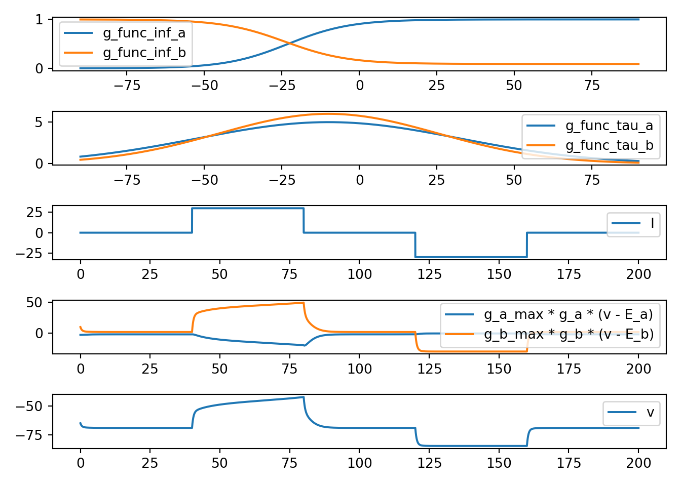
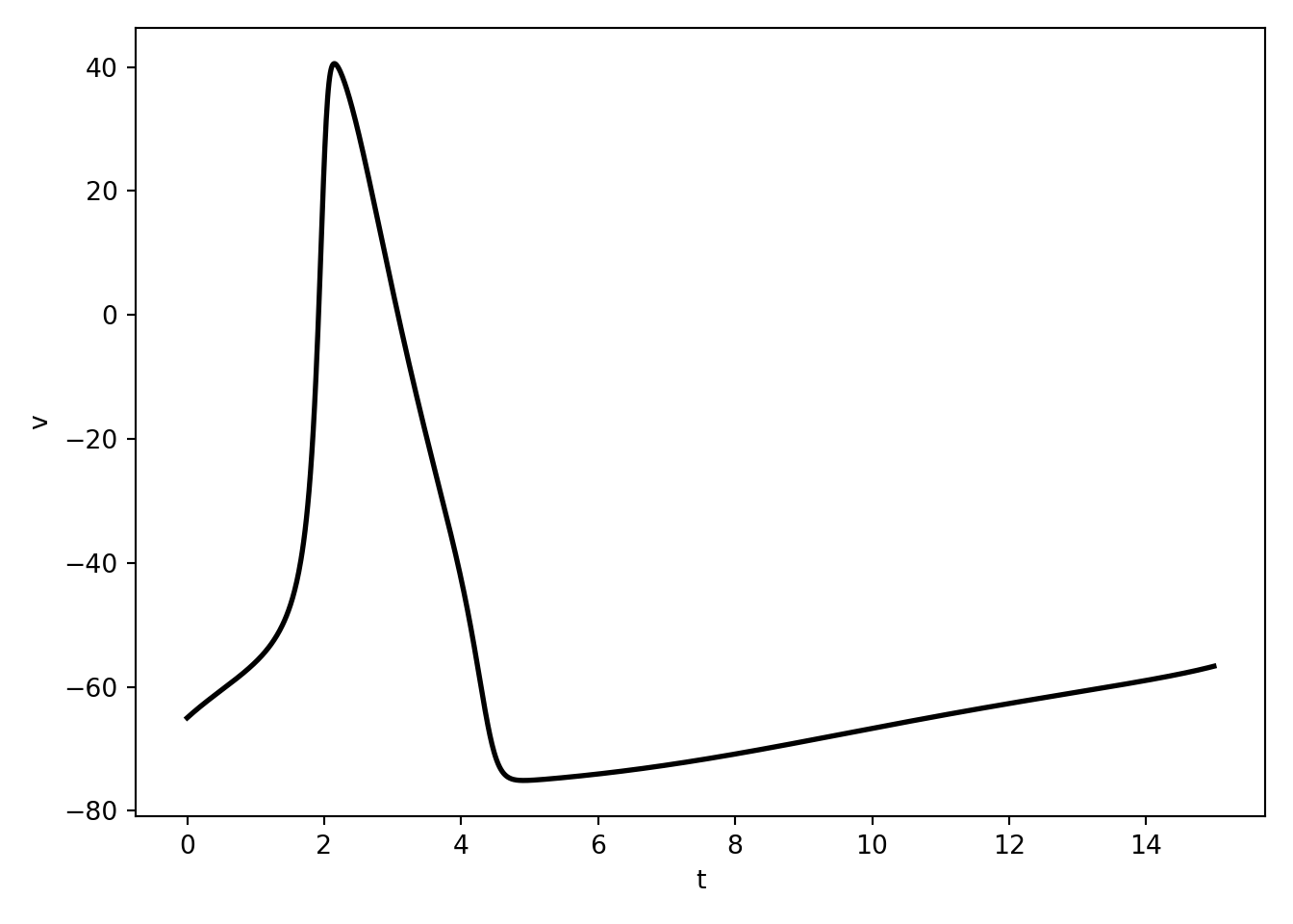
6.5 neuron_func_5
def neuron_func_5():
    '''
    dvdt = I - g_a_max * a_act**3 * a_inact * (v - E_a) - g_b * (v - E_b)
    dadt_act = (a_act_inf - a_act) / a_act_tau
    dadt_inact = (a_inact_inf - a_inact) / a_inact_tau
    - Increase due to I can be amplified
    - rise looks an action potential (due to a_act)
    - fall back to E_b (due to a_inact)
    - still not quite right... but why really?
    '''

    def g_func_inf_a_act(v):
        # sigmoid shape
        return 1 / (1 + 0.1 * np.exp(-0.5 * (v + 50.0)))

    def g_func_inf_a_inact(v):
        # sigmoid shape
        return -1 / (1.1 + 0.1 * np.exp(-0.1 * (v))) + 1

    def g_func_tau_a_act(v):
        # bell shape
        mu = -10.0
        sig = 60.0
        return (300 / sig) * np.exp(-((v - mu) / sig)**2)

    def g_func_tau_a_inact(v):
        # bell shape
        mu = -10.0
        sig = 50.0
        return (300 / sig) * np.exp(-((v - mu) / sig)**2)

    tau = 0.01
    T = 200
    t = np.arange(0, T, tau)
    n = t.shape[0]

    I = np.zeros(n)
    v = np.zeros(n)
    g_a_act = np.zeros(n)
    g_a_inact = np.zeros(n)

    vr = -65.0

    E_a = 120.0
    E_b = -70.0

    g_a_max = 2.0
    g_b_max = 1.0

    C = 1.0

    v[0] = vr
    g_a_act[0] = g_func_inf_a_act(vr)
    g_a_inact[0] = g_func_inf_a_inact(vr)

    I[n // 5:2 * n // 5] = 30.0
    I[3 * n // 5:4 * n // 5] = -30.0

    for i in range(1, n):
        delta_t = t[i] - t[i - 1]

        dvdt = (I[i - 1] - g_a_max * g_a_act[i - 1]**3 * g_a_inact[i - 1] *
                (v[i - 1] - E_a) - g_b_max * (v[i - 1] - E_b)) / C
        dgdt_a_act = (g_func_inf_a_act(v[i - 1]) -
                      g_a_act[i - 1]) / g_func_tau_a_act(v[i - 1])
        dgdt_a_inact = (g_func_inf_a_inact(v[i - 1]) -
                        g_a_inact[i - 1]) / g_func_tau_a_inact(v[i - 1])

        v[i] = v[i - 1] + dvdt * delta_t
        g_a_act[i] = g_a_act[i - 1] + dgdt_a_act * delta_t
        g_a_inact[i] = g_a_inact[i - 1] + dgdt_a_inact * delta_t

    fig, ax = plt.subplots(5, 1, squeeze=False)
    x = np.arange(-90, 90, 0.01)
    ax[0, 0].plot(x, g_func_inf_a_act(x), label='g_func_inf_a_act')
    ax[0, 0].plot(x, g_func_inf_a_inact(x), label='g_func_inf_a_inact')
    ax[1, 0].plot(x, g_func_tau_a_act(x), label='g_func_tau_a_act')
    ax[1, 0].plot(x, g_func_tau_a_inact(x), label='g_func_tau_a_inact')
    ax[2, 0].plot(t, I, label='I')
    ax[3, 0].plot(t,
                  g_a_max * g_a_act * (v - E_a),
                  label='g_a_max * g_a_act * (v - E_a)')
    ax[3, 0].plot(t,
                  g_a_max * g_a_inact * (v - E_a),
                  label='g_a_max * g_a_inact * (v - E_a)')
    ax[4, 0].plot(t, v, label='v')
    [x.legend() for x in ax.flatten()]
    plt.tight_layout()
    plt.show()

neuron_func_5()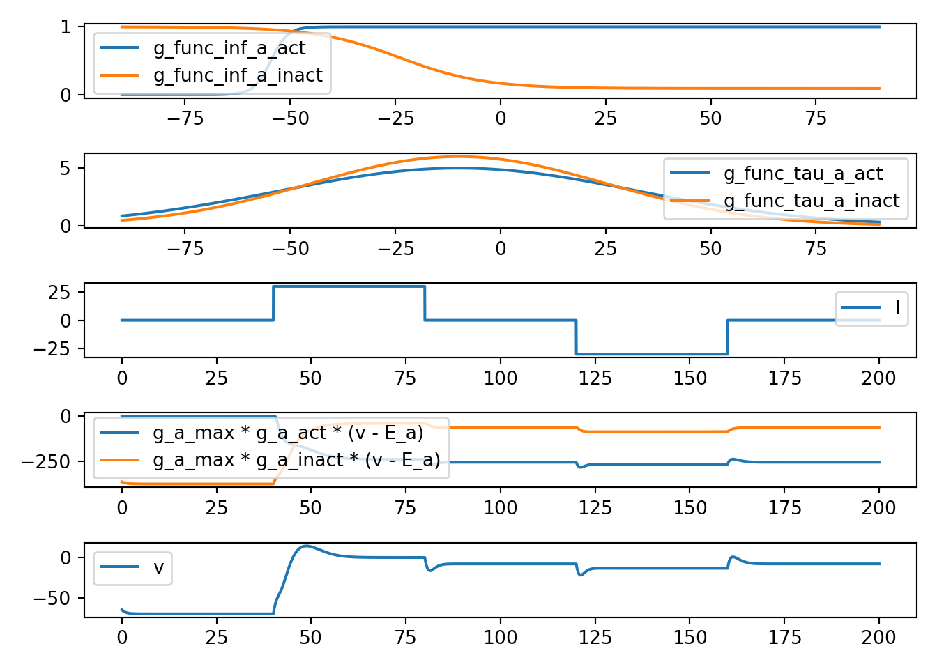
6.6 neuron_func_6
def neuron_func_6():
    '''
    dvdt = I - g_a_max * a_act**3 * a_inact * (v - E_a) - g_b_max * b * (v - E_b)
    dadt_act = (a_act_inf - a_act) / a_act_tau
    dadt_inact = (a_inact_inf - a_inact) / a_inact_tau
    dbdt = (b_inf - b) / b_tau
    - Increase due to I can be amplified
    - rise looks an action potential (due to a_act)
    - fall back to E_b (due to a_inact and due to b)
    - looking prettty good presumably
    '''

    def g_func_inf_a_act(v):
        # sigmoid shape
        return 1 / (1 + 0.1 * np.exp(-0.5 * (v + 50.0)))

    def g_func_inf_a_inact(v):
        # sigmoid shape
        return -1 / (1.1 + 0.1 * np.exp(-0.1 * (v))) + 1

    def g_func_inf_b(v):
        # sigmoid shape
        return 1 / (1.1 + 0.1 * np.exp(-0.09 * (v)))

    def g_func_tau_a_act(v):
        # bell shape
        mu = -10.0
        sig = 60.0
        return (300 / sig) * np.exp(-((v - mu) / sig)**2)

    def g_func_tau_a_inact(v):
        # bell shape
        mu = -10.0
        sig = 50.0
        return (300 / sig) * np.exp(-((v - mu) / sig)**2)

    def g_func_tau_b(v):
        # bell shape
        mu = 5.0
        sig = 50.0
        return (300 / sig) * np.exp(-((v - mu) / sig)**2)

    tau = 0.01
    T = 200
    t = np.arange(0, T, tau)
    n = t.shape[0]

    I = np.zeros(n)
    v = np.zeros(n)
    g_a_act = np.zeros(n)
    g_a_inact = np.zeros(n)
    g_b = np.zeros(n)

    vr = -65.0

    E_a = 120.0
    E_b = -70.0

    g_a_max = 2.0
    g_b_max = 5.0

    C = 1.0

    v[0] = vr
    g_a_act[0] = g_func_inf_a_act(vr)
    g_a_inact[0] = g_func_inf_a_inact(vr)
    g_b[0] = g_func_inf_b(vr)

    I[n // 5:2 * n // 5] = 30.0
    I[3 * n // 5:4 * n // 5] = -30.0

    for i in range(1, n):
        delta_t = t[i] - t[i - 1]

        dvdt = (I[i - 1] - g_a_max * g_a_act[i - 1]**3 * g_a_inact[i - 1] *
                (v[i - 1] - E_a) - g_b_max * g_b[i - 1]**4 *
                (v[i - 1] - E_b)) / C
        dgdt_a_act = (g_func_inf_a_act(v[i - 1]) -
                      g_a_act[i - 1]) / g_func_tau_a_act(v[i - 1])
        dgdt_a_inact = (g_func_inf_a_inact(v[i - 1]) -
                        g_a_inact[i - 1]) / g_func_tau_a_inact(v[i - 1])
        dgdt_b = (g_func_inf_b(v[i - 1]) - g_b[i - 1]) / g_func_tau_b(v[i - 1])

        v[i] = v[i - 1] + dvdt * delta_t
        g_a_act[i] = g_a_act[i - 1] + dgdt_a_act * delta_t
        g_a_inact[i] = g_a_inact[i - 1] + dgdt_a_inact * delta_t
        g_b[i] = g_b[i - 1] + dgdt_b * delta_t

    fig, ax = plt.subplots(5, 1, squeeze=False)
    x = np.arange(-90, 90, 0.01)
    ax[0, 0].plot(x, g_func_inf_a_act(x), label='g_func_inf_a_act')
    ax[0, 0].plot(x, g_func_inf_a_inact(x), label='g_func_inf_a_inact')
    ax[0, 0].plot(x, g_func_inf_b(x), label='g_func_inf_b')
    ax[1, 0].plot(x, g_func_tau_a_act(x), label='g_func_tau_a_act')
    ax[1, 0].plot(x, g_func_tau_a_inact(x), label='g_func_tau_a_inact')
    ax[1, 0].plot(x, g_func_tau_b(x), label='g_func_tau_b')
    ax[2, 0].plot(t, I, label='I')
    ax[3, 0].plot(t,
                  g_a_max * g_a_act * (v - E_a),
                  label='g_a_max * g_a_act * (v - E_a)')
    ax[3, 0].plot(t,
                  g_a_max * g_a_inact * (v - E_a),
                  label='g_a_max * g_a_inact * (v - E_a)')
    ax[3, 0].plot(t,
                  g_b_max * g_b * (v - E_b),
                  label='g_b_max * g_b * (v - E_b)')
    ax[4, 0].plot(t, v, label='v')
    [x.legend() for x in ax.flatten()]
    plt.tight_layout()
    plt.show()

neuron_func_6()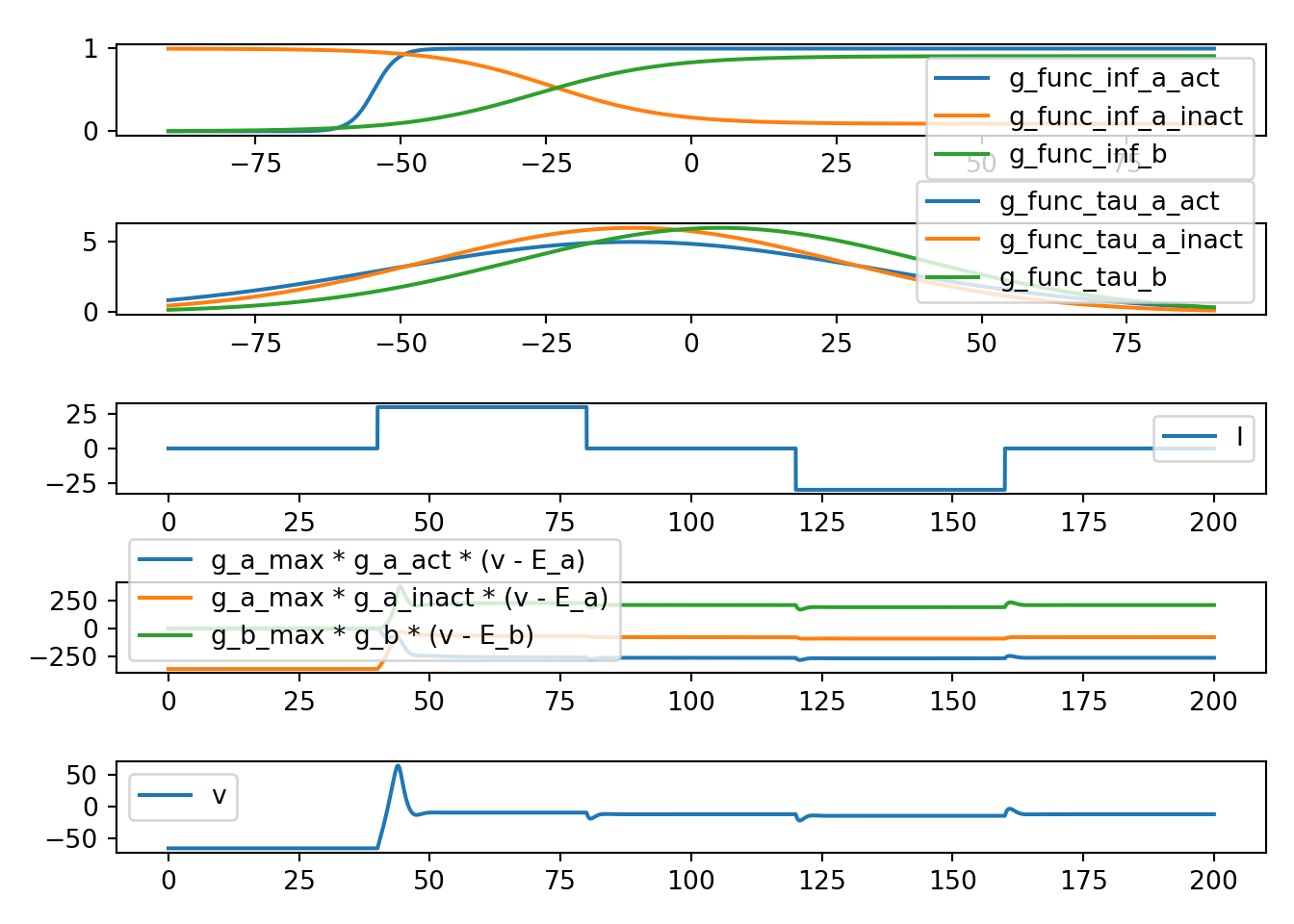
6.7 neuron_func_7
def neuron_func_7():
    '''
    NOTE: Full HH
    '''

    # NOTE: n gating variables
    def n_inf(v):
        return alpha_func_n(v) / (alpha_func_n(v) + beta_func_n(v))

    def n_tau(v):
        return 1.0 / (alpha_func_n(v) + beta_func_n(v))

    def alpha_func_n(v):
        return 0.01 * (10.0 - v) / (np.exp((10.0 - v) / 10.0) - 1.0)

    def beta_func_n(v):
        return 0.125 * np.exp(-v / 80.0)

    # NOTE: m gating variables
    def m_inf(v):
        return alpha_func_m(v) / (alpha_func_m(v) + beta_func_m(v))

    def m_tau(v):
        return 1.0 / (alpha_func_m(v) + beta_func_m(v))

    def alpha_func_m(v):
        return 0.1 * (25.0 - v) / (np.exp((25.0 - v) / 10.0) - 1.0)

    def beta_func_m(v):
        return 4.0 * np.exp(-v / 18.0)

    # NOTE: h gating variables
    def h_inf(v):
        return alpha_func_h(v) / (alpha_func_h(v) + beta_func_h(v))

    def h_tau(v):
        return 1.0 / (alpha_func_h(v) + beta_func_h(v))

    def alpha_func_h(v):
        return 0.07 * np.exp(-v / 20.0)

    def beta_func_h(v):
        return 1.0 / (np.exp((30.0 - v) / 10.0) + 1.0)

    # NOTE: simulation parameter etc
    tau = 0.01
    T = 200
    t = np.arange(0, T, tau)
    nn = t.shape[0]

    I = np.zeros(nn)
    v = np.zeros(nn)
    n = np.zeros(nn)
    m = np.zeros(nn)
    h = np.zeros(nn)

    vr = -65.0

    v[0] = vr
    n[0] = n_inf(vr*0)
    m[0] = m_inf(vr*0)
    h[0] = h_inf(vr*0)

    g_k = 36.0
    g_na = 120.0
    g_leak = 0.30

    E_k = -12 + vr
    E_na = 120 + vr
    E_leak = 10.6 + vr

    C = 1.0

    I[nn // 5:2 * nn // 5] = 5.0
    I[3 * nn // 5:4 * nn // 5] = -5.0

    # NOTE: Euler's method simulation
    for i in range(1, nn):
        delta_t = t[i] - t[i - 1]

        I_k = g_k * (n[i - 1]**4) * (v[i - 1] - E_k)
        I_na = g_na * (m[i - 1]**3) * (h[i - 1]) * (v[i - 1] - E_na)
        I_leak = g_leak * (v[i - 1] - E_leak)

        dvdt = (I[i - 1] - (I_k + I_na + I_leak)) / C

        dndt = (n_inf(v[i - 1] - vr) - n[i - 1]) / n_tau(v[i - 1] - vr)
        dmdt = (m_inf(v[i - 1] - vr) - m[i - 1]) / m_tau(v[i - 1] - vr)
        dhdt = (h_inf(v[i - 1] - vr) - h[i - 1]) / h_tau(v[i - 1] - vr)

        v[i] = v[i - 1] + dvdt * delta_t
        n[i] = n[i - 1] + dndt * delta_t
        m[i] = m[i - 1] + dmdt * delta_t
        h[i] = h[i - 1] + dhdt * delta_t

    # NOTE: inspect gating functions
    fig, ax = plt.subplots(5, 1, squeeze=False)

    v_range = np.arange(-40, 100, 0.01)

    ax[0, 0].plot(v_range, n_inf(v_range), label='n: k activation')
    ax[0, 0].plot(v_range, m_inf(v_range), label='m: Na activation')
    ax[0, 0].plot(v_range, h_inf(v_range), label='h: Na inactivation')
    ax[1, 0].plot(v_range, n_tau(v_range), label='n: k activation')
    ax[1, 0].plot(v_range, m_tau(v_range), label='m: Na activation')
    ax[1, 0].plot(v_range, h_tau(v_range), label='h: Na inactivation')
    ax[2, 0].plot(t, I, label='I')
    ax[3, 0].plot(t, v, label='v')
    ax[4, 0].plot(t, n, label='n: k activation')
    ax[4, 0].plot(t, m, label='m: Na activation')
    ax[4, 0].plot(t, h, label='h: Na inactivation')
    [x.legend() for x in ax.flatten()]
    plt.tight_layout()
    plt.show()

neuron_func_7()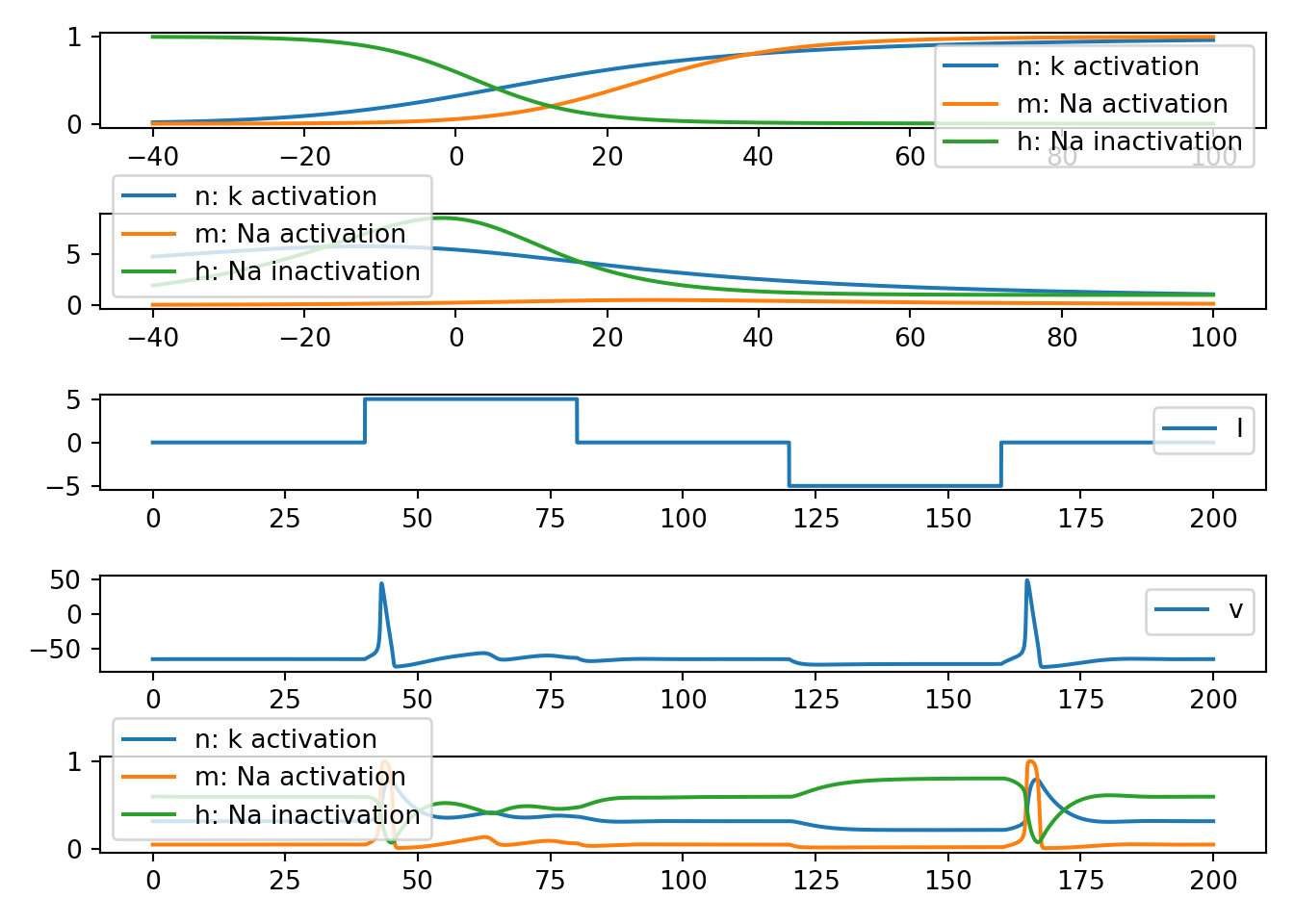
6.8 Review of HH
\[ C \frac{d}{dt}V = I - \overline{g}_{K} n^4 (V - E_{K}) - \overline{g}_{Na} m^3 h (V - E_{Na}) - \overline{g}_{L} (V - E_{L})\\ \frac{d}{dt}n = (n_{\infty}(V) - n) / \tau(V) \\ \frac{d}{dt}m = (m_{\infty}(V) - m) / \tau(V) \\ \frac{d}{dt}h = (h_{\infty}(V) - h) / \tau(V) \\ \]
HH model is an example of a conductance-based model
One advantage of conductance-based models is that their parameters have well-defined biophysical meanings.
However, this does not mean that measuring the true value of these parameters is easy. Rather, it is often difficult and noisy.
Furthermore, it is difficult to ensure the model will behave like a real neuron outside the stimulation protocols used to measure model parameters.